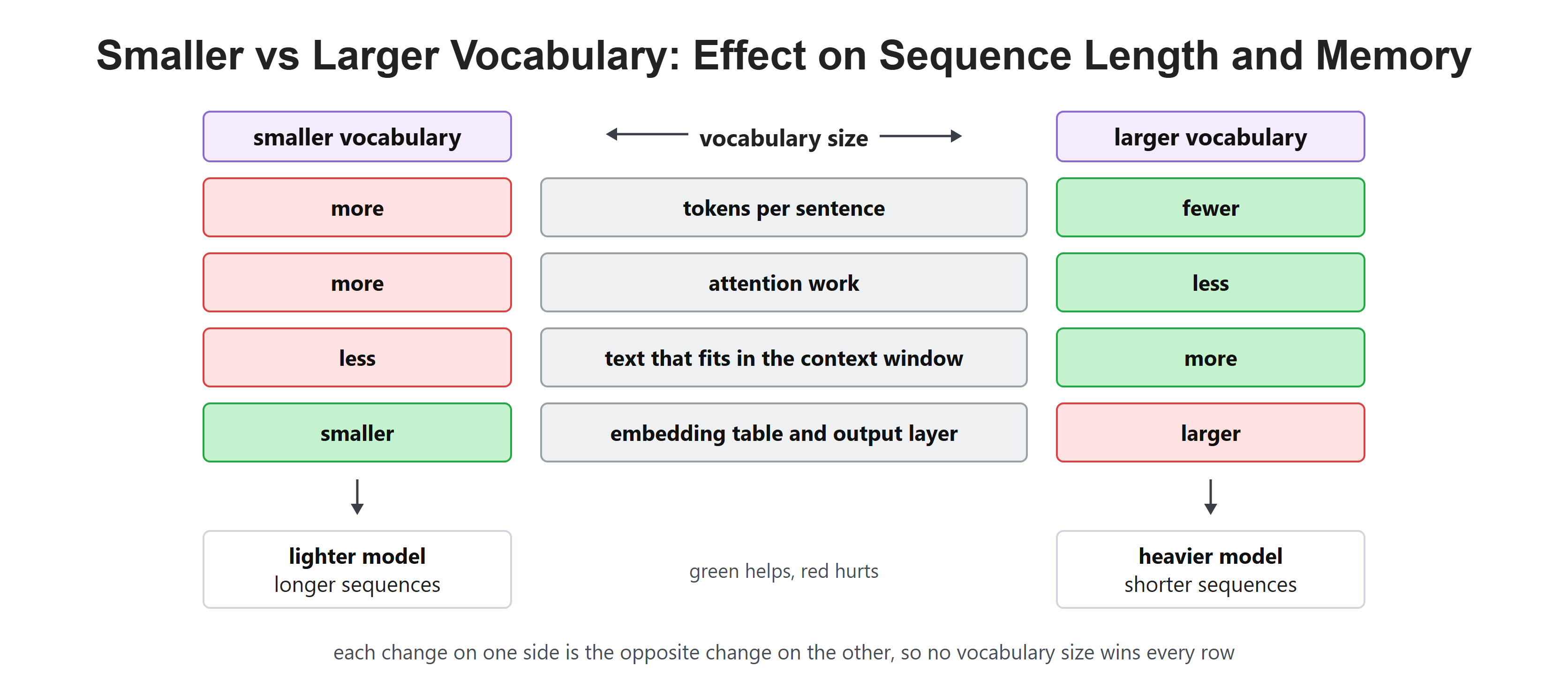
Every tokenizer has one dial we can turn: how many tokens to keep in the vocabulary. Turn it up and each sentence needs fewer tokens. Turn it down and the model gets lighter.
We cannot have both. This is the central trade-off of tokenization, and it quietly shapes how long our prompts can be and how much memory a model needs. In this blog, we will learn what each side of the dial costs and where real models set it.
The Same Sentence, Two Vocabularies
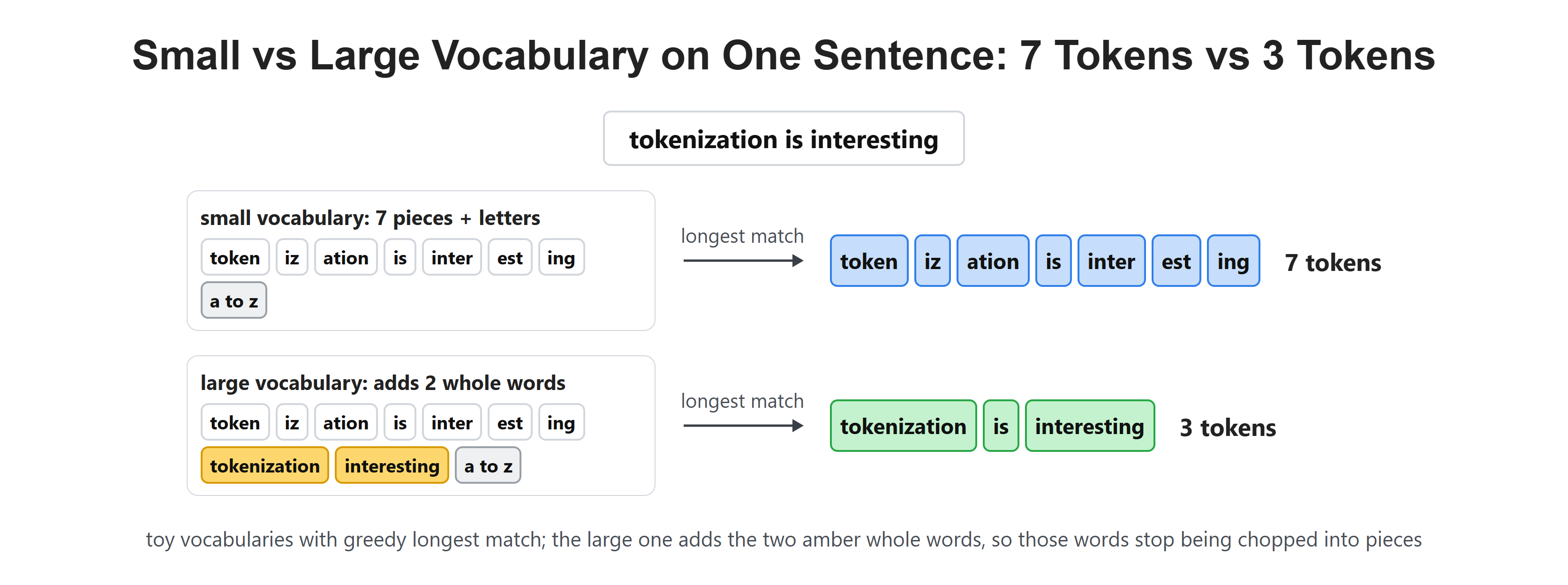
We start with the effect we can see. Let's say we take one sentence and tokenize it twice, once with a small vocabulary and once with a large one.
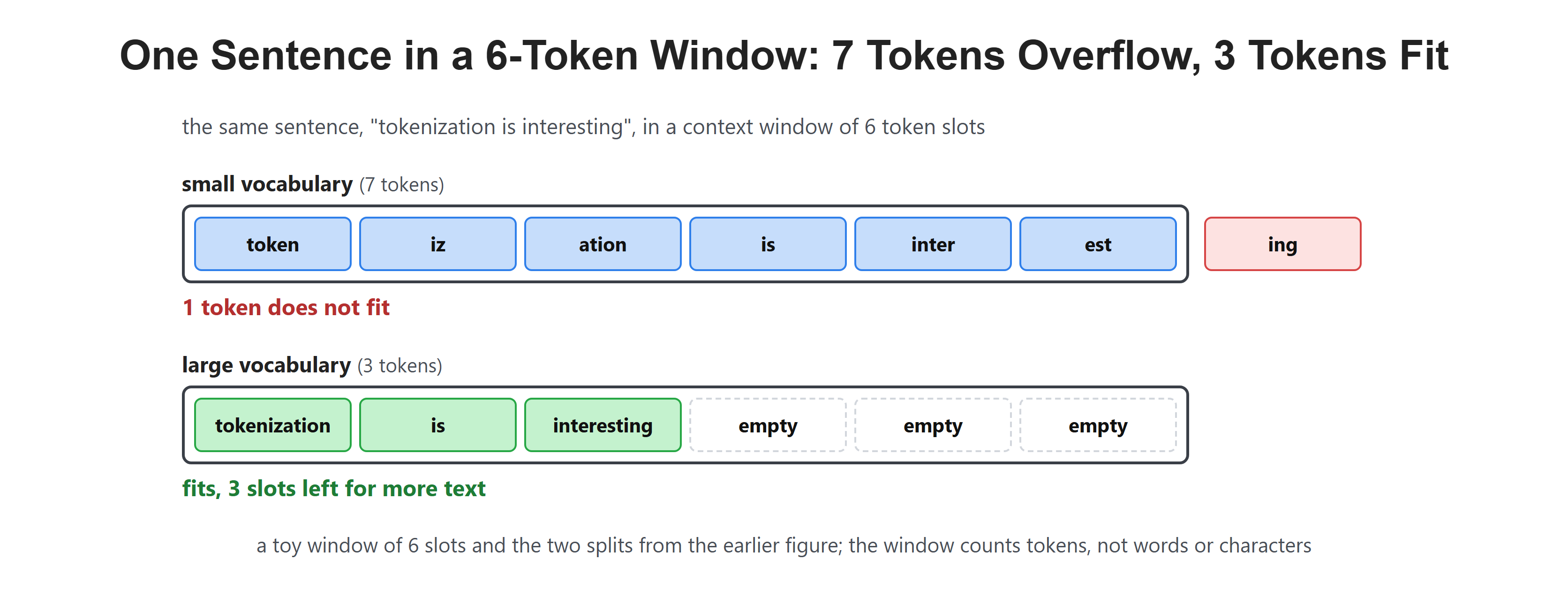
With a small vocabulary the model has few whole words, so it must chop text into many small pieces. With a large vocabulary, many words already exist as single tokens. So the same sentence becomes a much shorter list. In the figure, it drops from 7 tokens to 3.
Why Shorter Sequences Matter So Much
Fewer tokens is not just tidier. It changes what the model can do and what it costs.
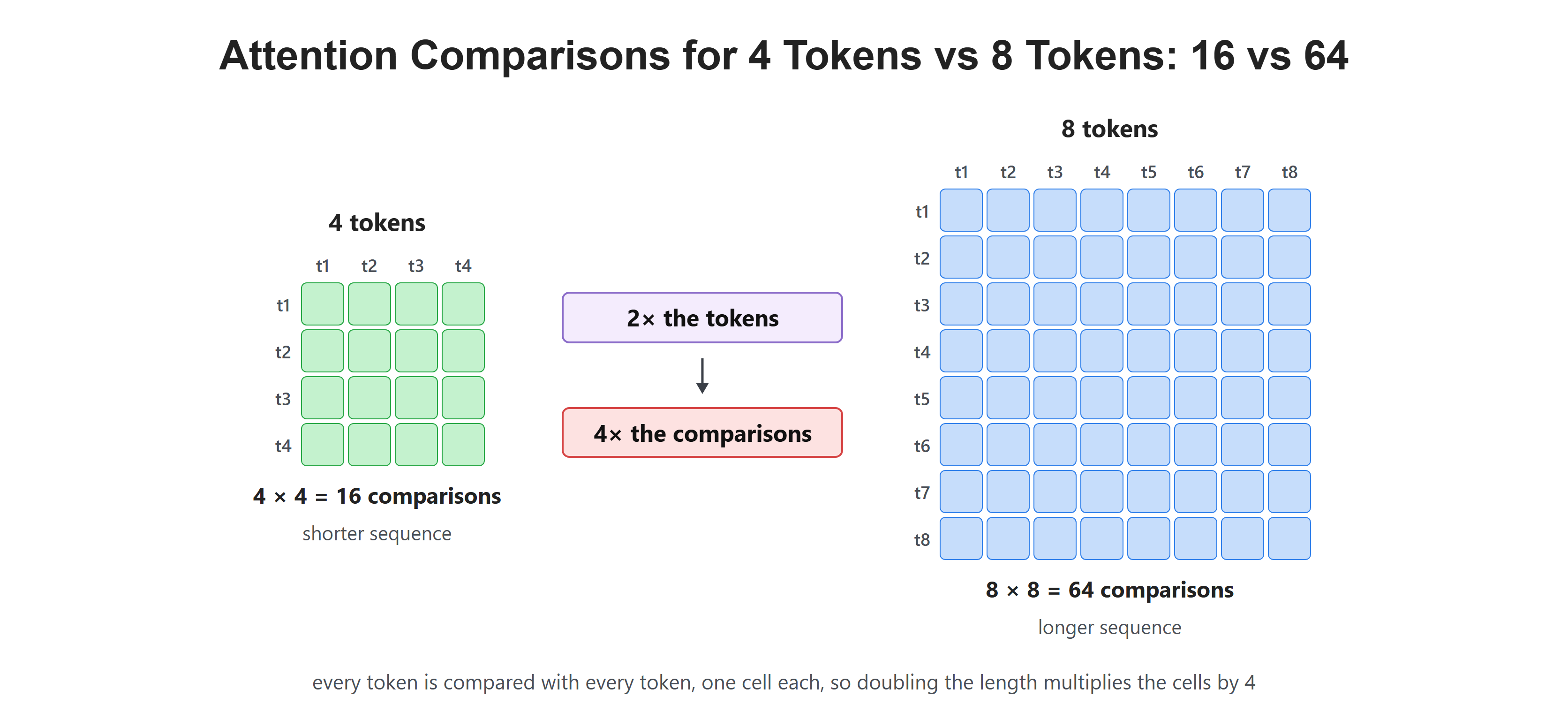
Attention compares every token with every other token. Double the tokens and the attention work grows roughly four times, not two: 4 tokens need 16 comparisons, while 8 tokens need 64. This square growth applies to attention only, not to the whole model. Even so, it means a shorter sequence makes attention much cheaper.
Shorter sequences also mean more real text fits inside the context window, and for paid APIs, fewer tokens means a smaller bill.
What a Bigger Vocabulary Costs
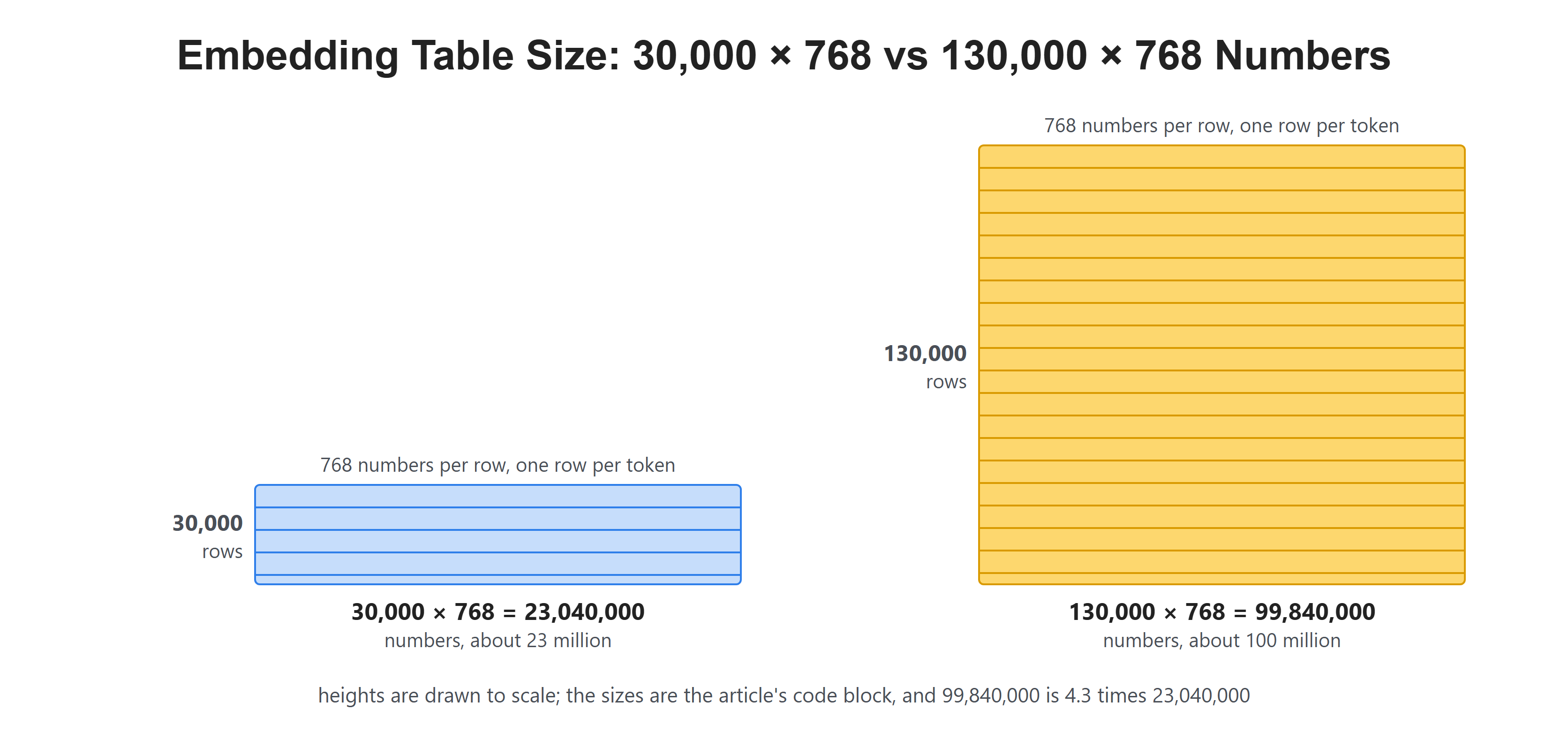
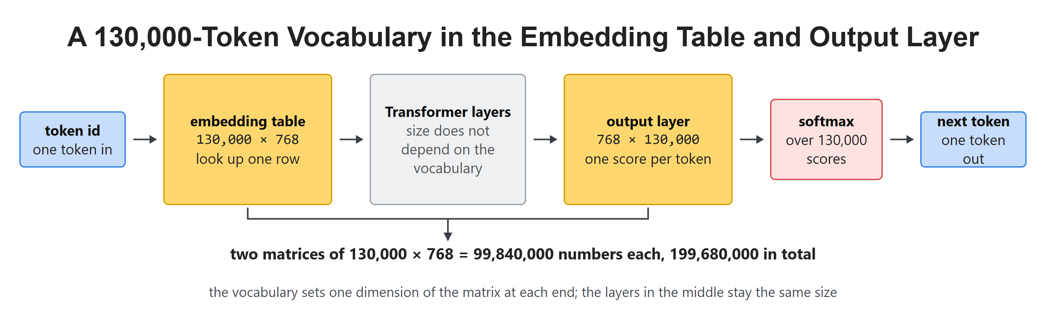
Now the other side. Every token in the vocabulary needs its own row in the embedding table. Each row is a vector with one number per dimension.
So the table's size is vocabulary size multiplied by embedding dimension. Grow the vocabulary and that table grows in a straight line, taking memory with it. In the code below, we use 768 dimensions, the hidden size of BERT-base and GPT-2 small:
# embedding table size = vocab_size x hidden_dim
# 30,000 x 768   -> about 23 million numbers
# 130,000 x 768  -> about 100 million numbers
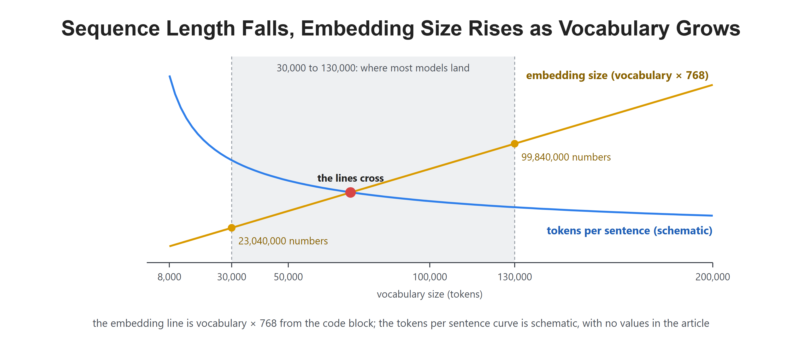
Here, we can see that 30,000 × 768 is 23,040,000 numbers, while 130,000 × 768 is 99,840,000 numbers.
The Output Layer Pays Twice
The cost does not stop at the input. At the other end of the model, the final layer must produce a score for every token in the vocabulary, so it can pick the next word.
That means a second big matrix of the same size, 768 × 130,000 in our example. Two such matrices hold 199,680,000 numbers in total. A larger vocabulary makes both ends of the model heavier, and it makes the final softmax slower.
Many models save some of this by sharing one matrix between the embedding table and the output layer. This is called weight tying, and GPT-2 does it. Models that tie weights store the matrix only once.
The Context Window Is Counted in Tokens
Here is where the trade-off becomes visible to users. A model's context window is a fixed number of tokens, not words and not characters.
So the same document can fit or overflow depending purely on the tokenizer. In a 6-token window, our sentence overflows at 7 tokens but fits at 3. An efficient tokenizer packs more real text into the same window.
Why This Hits Other Languages Hardest
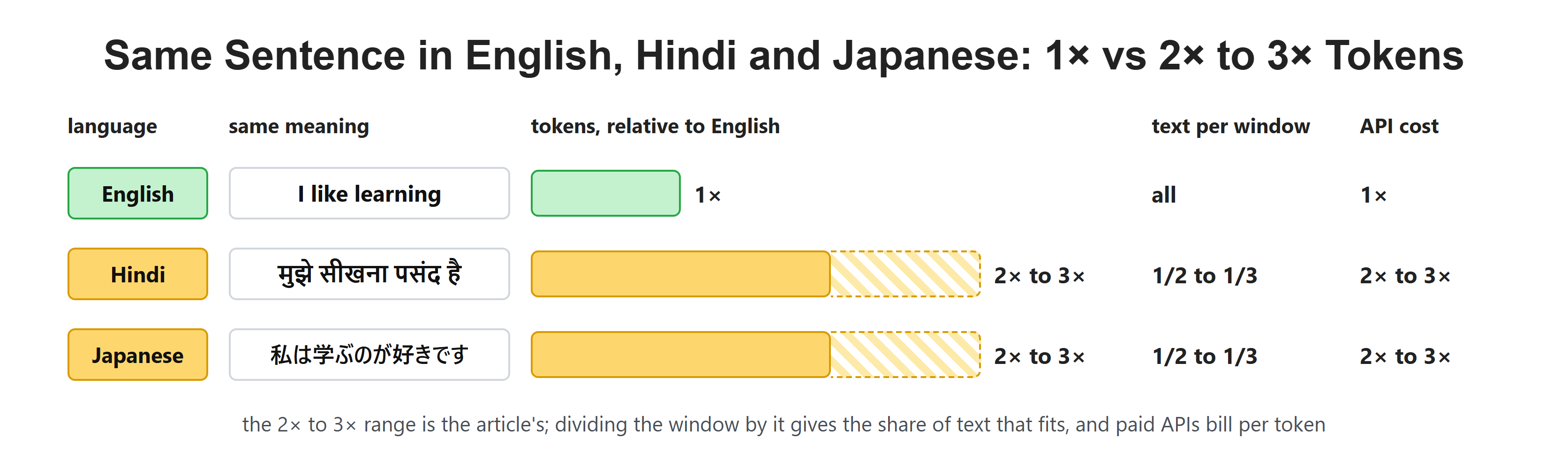
Most tokenizers are trained mainly on English, so English words tend to be single tokens. Other languages get chopped into many small pieces.
As a result, the same sentence in Hindi or Japanese can take two to three times as many tokens with a tokenizer trained mostly on English. The exact gap depends on the tokenizer. The window holds less text, and on a paid API the cost rises, for the same meaning.
Where Real Models Land
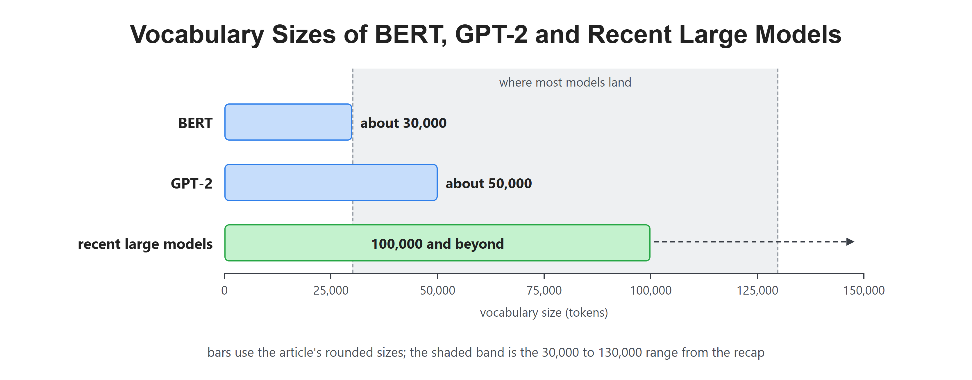
Given both pressures, most models settle in a familiar band. BERT used about 30,000 tokens (30,522 exactly). GPT-2 used about 50,000 (50,257 exactly). Recent large models have pushed to 100,000 and beyond, partly to handle many languages and code more fairly.
The trend has been upward, because memory has grown cheaper while long context has grown more valuable.
How the Dial Is Actually Chosen
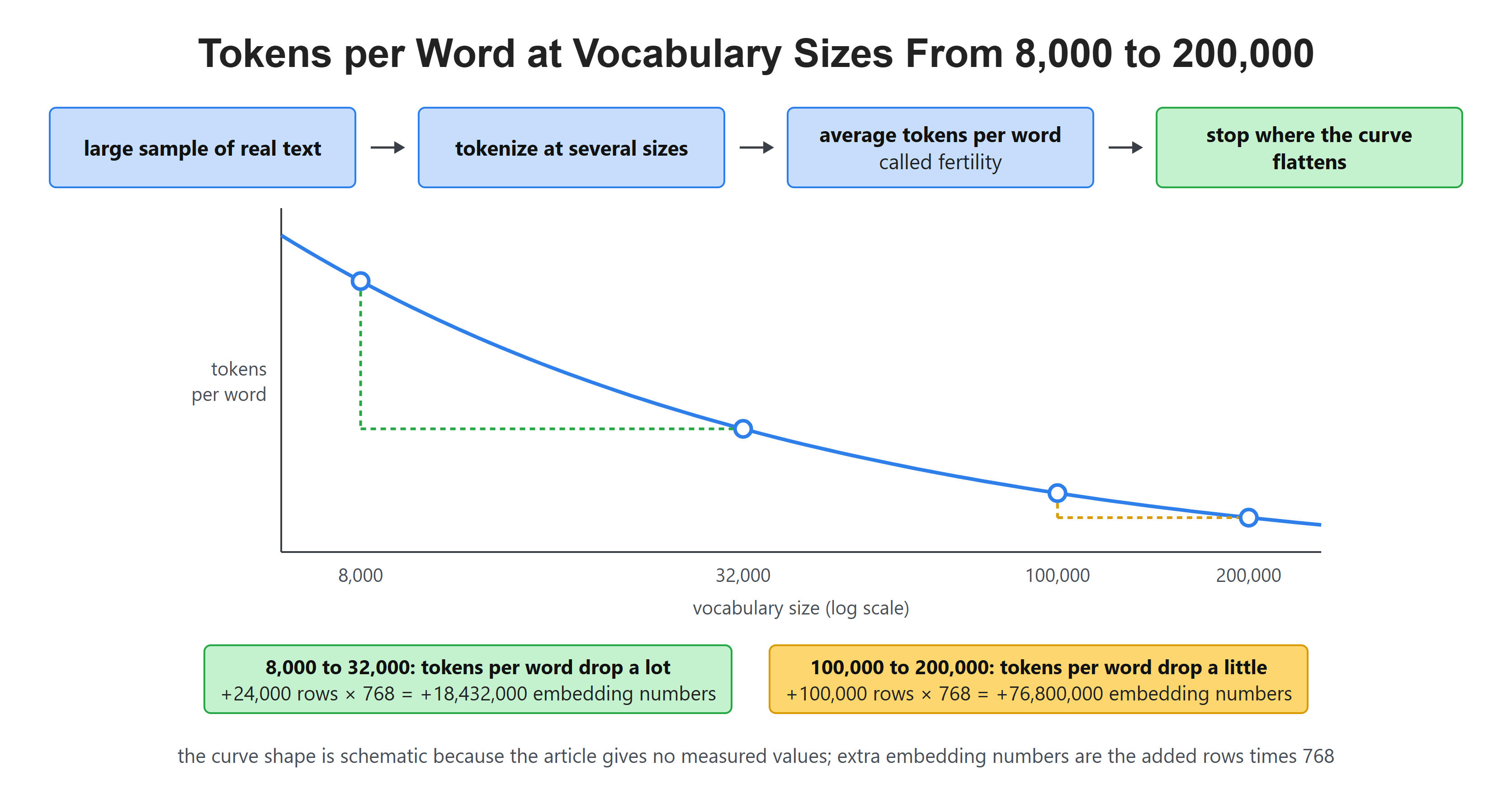
Nobody picks the number by feel. Teams tokenize a large sample of their real text at several vocabulary sizes. Then they measure the average tokens per word, sometimes called fertility.
The curve flattens. Going from 8,000 to 32,000 tokens cuts tokens per word a lot. With 768 numbers per row, it adds 24,000 × 768 = 18,432,000 embedding numbers. Going from 100,000 to 200,000 cuts tokens per word only a little, yet it adds 100,000 × 768 = 76,800,000 numbers. So the gain shrinks while the memory cost grows. Teams stop where the curve stops paying.
The Trade-Off in One Picture
Put the two costs together and the shape becomes clear. Sequence length falls as vocabulary grows, while memory rises. The tokens-per-sentence curve is only a sketch, so the point where the lines cross is not a measured number. The idea is what matters: the best choice sits in the middle, not at either extreme. Most models land between 30,000 and 130,000 tokens.
Recap
This is how the vocabulary size vs context window trade-off works. A bigger vocabulary turns each sentence into fewer tokens. That saves attention work, fits more text in the context window, and lowers cost. But every extra token needs a row in the embedding table and a slot in the output layer, so memory rises in a straight line.
The context window is measured in tokens, so the tokenizer decides how much real text fits. Languages that were under-represented during training pay more for the same meaning. Most models land between 30,000 and 130,000 tokens, chosen by measuring where the savings curve flattens.
In the next article, we look at what happens when tokenization gets strange. We will see why a model that can write an essay cannot reliably count the letter R in the word strawberry.