Qwen2.5-0.5B is the smallest model in the Qwen2.5 family, which Alibaba's Qwen team released in September 2024. It has 494M parameters and runs on almost any GPU. But inside that small file sits the same machine as the big chat models: a decoder that reads tokens and scores every possible next token.
In this blog, we will learn how Qwen2.5-0.5B works by running real code on it. We will follow one short sentence from text to tokens, through 24 decoder layers, to the next-token scores. On the way, we will see what each part does, where the weights sit and how much memory generation needs.
What Is Qwen2.5-0.5B?
Qwen2.5 is built on the Transformer, the design from the 2017 paper "Attention Is All You Need" by Vaswani et al. So before we open Qwen, let's look at that original model as below.
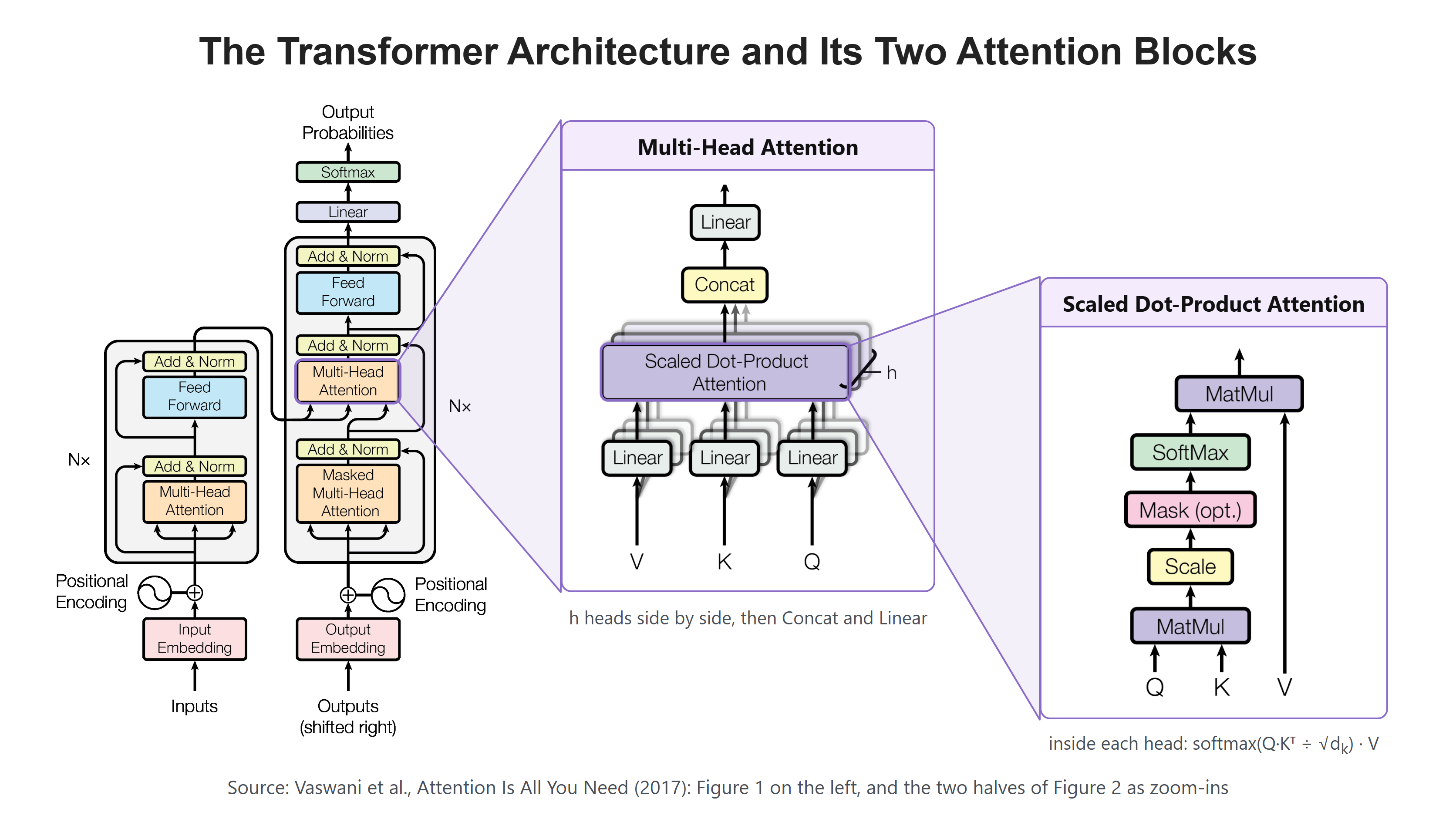
Here, we can see two towers. The left tower is the encoder, which reads the whole input at once. The right tower is the decoder. Its Masked Multi-Head Attention lets each token look only at the tokens before it, and its Linear and Softmax at the top score the next token. Qwen2.5 keeps only the decoder tower and drops the middle attention block that reads from the encoder. The "Nx" next to the tower means the layer is stacked N times, and in Qwen2.5-0.5B N is 24. The two zoom-ins on the right show Multi-Head Attention and the Scaled Dot-Product Attention inside each head, and Qwen still runs that same attention in every layer.
The Qwen2.5 family comes in seven sizes, from 0.5B to 72B parameters. All of them are dense, decoder-only models, pretrained on up to 18 trillion tokens. The 0.5B model is released under the Apache 2.0 license, and its model card lists a context length of 32,768 tokens.
Each size ships as a base model and an instruct model. The base model only continues text. The instruct model is the same network, trained further to follow chat instructions. In this blog, we use Qwen2.5-0.5B-Instruct, the model our course notebook uses. The base model has the same architecture, so every shape and weight count below applies to it too.
Let me tabulate the main settings for your better understanding.
| Setting | Value |
|---|---|
| Parameters | 494,032,768 (0.49B) |
| Parameters without embeddings | 357,898,112 (0.36B) |
| Decoder layers | 24 |
| Hidden size (numbers per token) | 896 |
| Query heads | 14 |
| Key and value heads | 2 |
| Head size | 64 |
| MLP size | 4,864 |
| Embedding rows | 151,936 |
| Tokenizer entries | 151,665 |
| Context length | 32,768 tokens |
| Positions | RoPE, base 1,000,000 |
| Norm | RMSNorm, eps 1e-6 |
| MLP activation | SiLU, inside a SwiGLU MLP |
| LM head | Shared with the embedding table |
| Stored weights | bfloat16 |
The picture below shows the whole model at once. On the left is the full stack: a token embedding, 24 decoder layers, a final RMSNorm and the LM head. The middle panel zooms into one decoder layer, and the right panels zoom into its MLP and its attention.
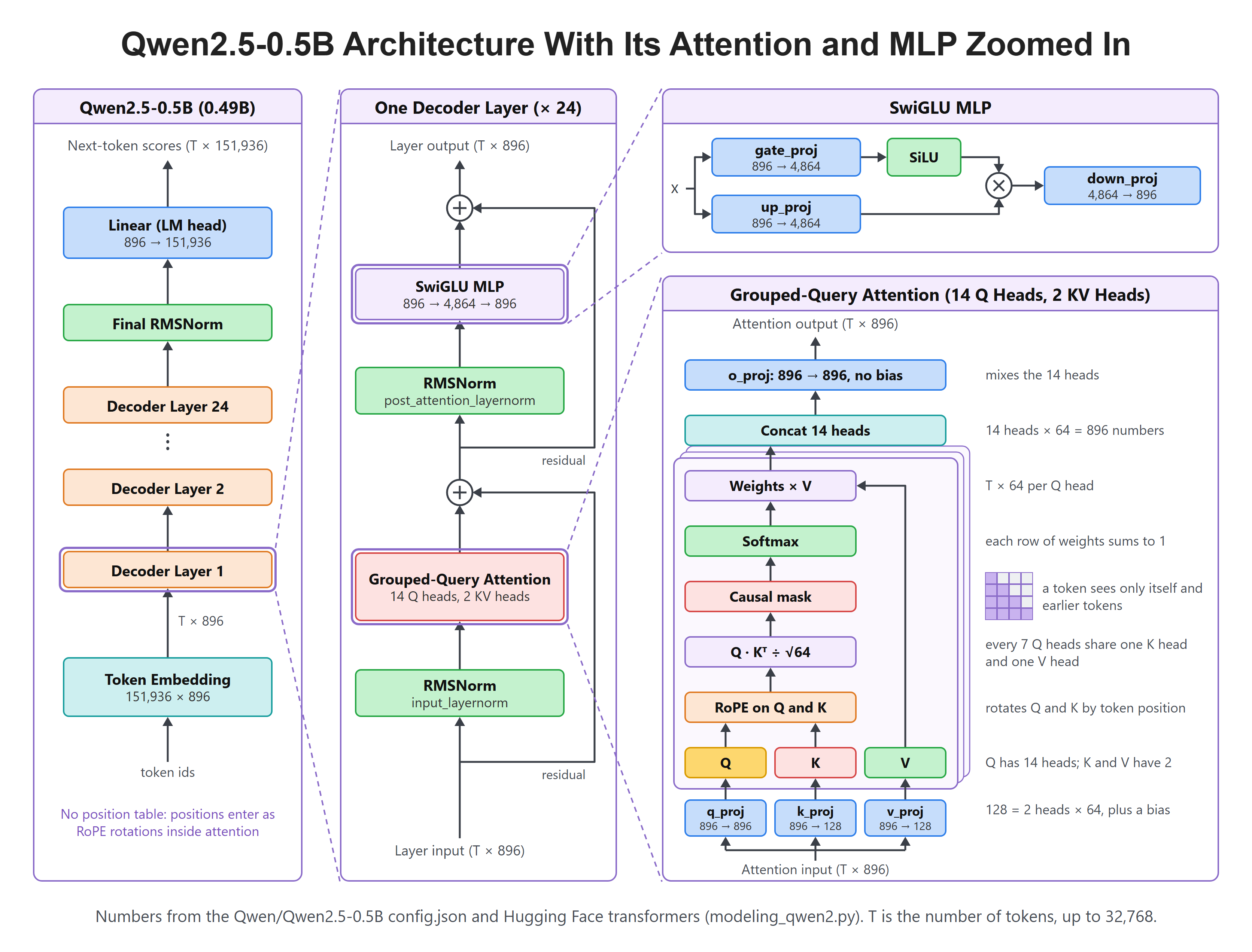
Here, we can see two things that stand out. There is no position table at the bottom of the model, because positions enter as RoPE rotations inside attention. And attention makes only 2 key heads and 2 value heads for its 14 query heads. We will open every one of these boxes with code.
Qwen2.5 keeps the plan of the original Transformer's decoder: a stack of identical layers, each with masked self-attention and an MLP, joined by residual connections. But four parts inside the layer are newer than the 2017 paper: RMSNorm, RoPE, grouped-query attention and SwiGLU. We will meet each one below.
Our Test Setup
We run every example on one NVIDIA GeForce RTX 5090 (32 GB) with PyTorch 2.11.0 and Hugging Face transformers 5.2.0. The model loads in its stored format, bfloat16. We never train anything, so gradients are switched off for the whole blog.
Every number in this blog, and in every figure, comes from the code below. The examples follow the course notebook: the same sentences, the same random seed and the same order of steps.
Let's see the code as below. It loads the tokenizer and the model, then prints the model:
import math
import torch
import matplotlib.pyplot as plt
from transformers import AutoTokenizer, AutoModelForCausalLM, logging

torch.set_grad_enabled(False)
logging.set_verbosity_error()

MODEL = "Qwen/Qwen2.5-0.5B-Instruct"

tok = AutoTokenizer.from_pretrained(MODEL)
model = AutoModelForCausalLM.from_pretrained(MODEL, device_map="cuda")
modelQwen2ForCausalLM(
(model): Qwen2Model(
(embed_tokens): Embedding(151936, 896)
(layers): ModuleList(
(0-23): 24 x Qwen2DecoderLayer(
(self_attn): Qwen2Attention(
(q_proj): Linear(in_features=896, out_features=896, bias=True)
(k_proj): Linear(in_features=896, out_features=128, bias=True)
(v_proj): Linear(in_features=896, out_features=128, bias=True)
(o_proj): Linear(in_features=896, out_features=896, bias=False)
)
(mlp): Qwen2MLP(
(gate_proj): Linear(in_features=896, out_features=4864, bias=False)
(up_proj): Linear(in_features=896, out_features=4864, bias=False)
(down_proj): Linear(in_features=4864, out_features=896, bias=False)
(act_fn): SiLUActivation()
)
(input_layernorm): Qwen2RMSNorm((896,), eps=1e-06)
(post_attention_layernorm): Qwen2RMSNorm((896,), eps=1e-06)
)
)
(norm): Qwen2RMSNorm((896,), eps=1e-06)
(rotary_emb): Qwen2RotaryEmbedding()
)
(lm_head): Linear(in_features=896, out_features=151936, bias=False)
)Here, we can see the whole model in a few lines. embed_tokens is the table of 151,936 token vectors. layers holds 24 copies of the same decoder layer, each with self_attn, mlp and two Qwen2RMSNorm layers. At the end, norm is the final RMSNorm and lm_head turns each vector of 896 numbers into 151,936 scores. rotary_emb holds no weights: it only computes rotation angles.
The config gives us the head counts and the MLP size directly.
model.config.num_attention_heads, model.config.num_key_value_heads, model.config.intermediate_size(14, 2, 4864)So every layer has 14 query heads, only 2 key-value heads, and an MLP that widens 896 numbers to 4,864.
How Does Text Become Tokens?
The model never sees letters or words. It only sees token ids, which are row numbers in its vocabulary. Qwen2.5 uses a byte-level BPE tokenizer, so any text, in any language, can be split into tokens it knows.
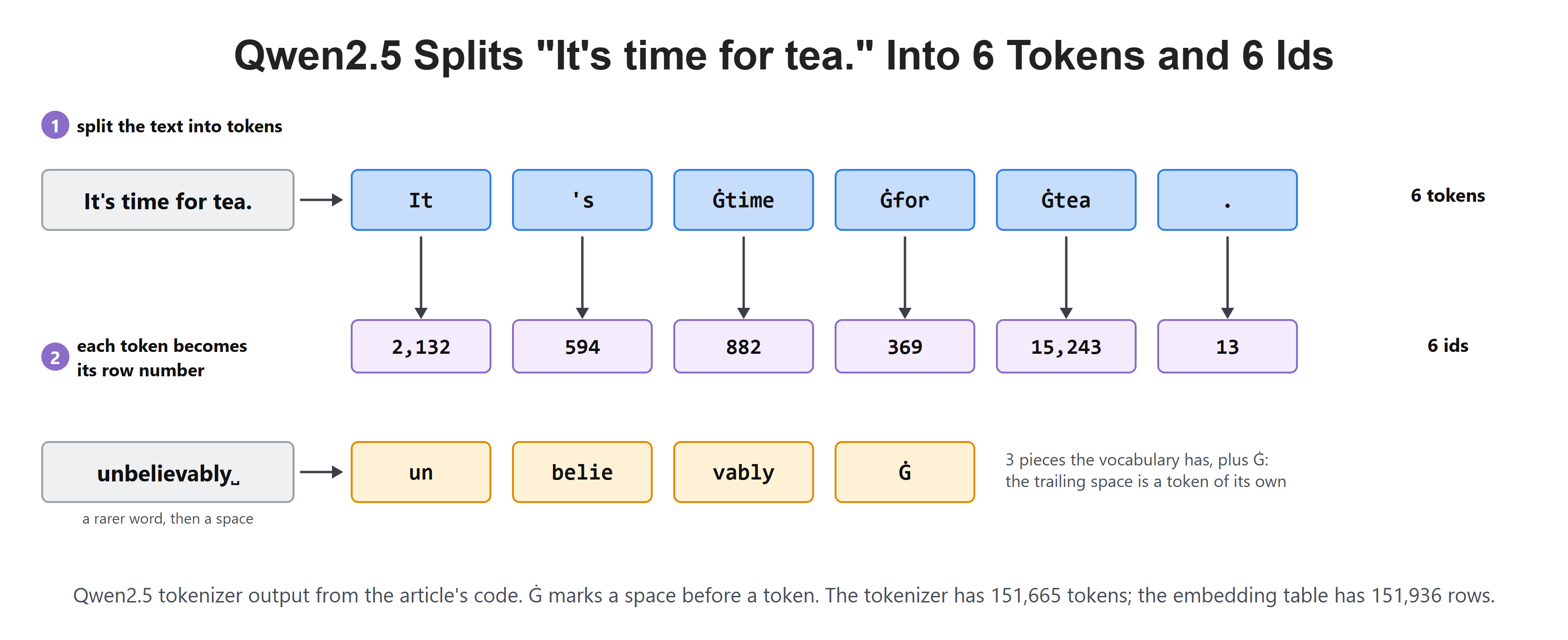
The figure below shows the two examples we will run. "It's time for tea." splits into 6 tokens, and each token becomes its row number in the vocabulary, its id. The rarer word "unbelievably" splits into 3 pieces plus a space.
Let's tokenize the notebook's first sentence.
ids = tok("It's time for tea.")["input_ids"]
ids[2132, 594, 882, 369, 15243, 13]The sentence becomes 6 ids. To see what each id stands for, we turn them back into tokens.
tok.convert_ids_to_tokens(ids)['It', "'s", 'Ġtime', 'Ġfor', 'Ġtea', '.']Here, we can see 6 tokens. Ġ is how the tokenizer prints a space, so Ġtea means " tea" with its leading space. Common words are one token each.
A rarer word splits into pieces that the vocabulary does have.
tok.convert_ids_to_tokens(tok("unbelievably ")["input_ids"])['un', 'belie', 'vably', 'Ġ']Here, "unbelievably" becomes 3 pieces, and the trailing space becomes a token of its own.
Now let's count the tokenizer's entries.
len(tok)151665The tokenizer has 151,665 entries: 151,643 learned by BPE and 22 special tokens, such as the markers of the chat template.
How Do Token Ids Become Vectors?
Each token id picks one row of a large learned table, the embedding table. That row is the token's first vector, and it is what the 24 layers will work on.
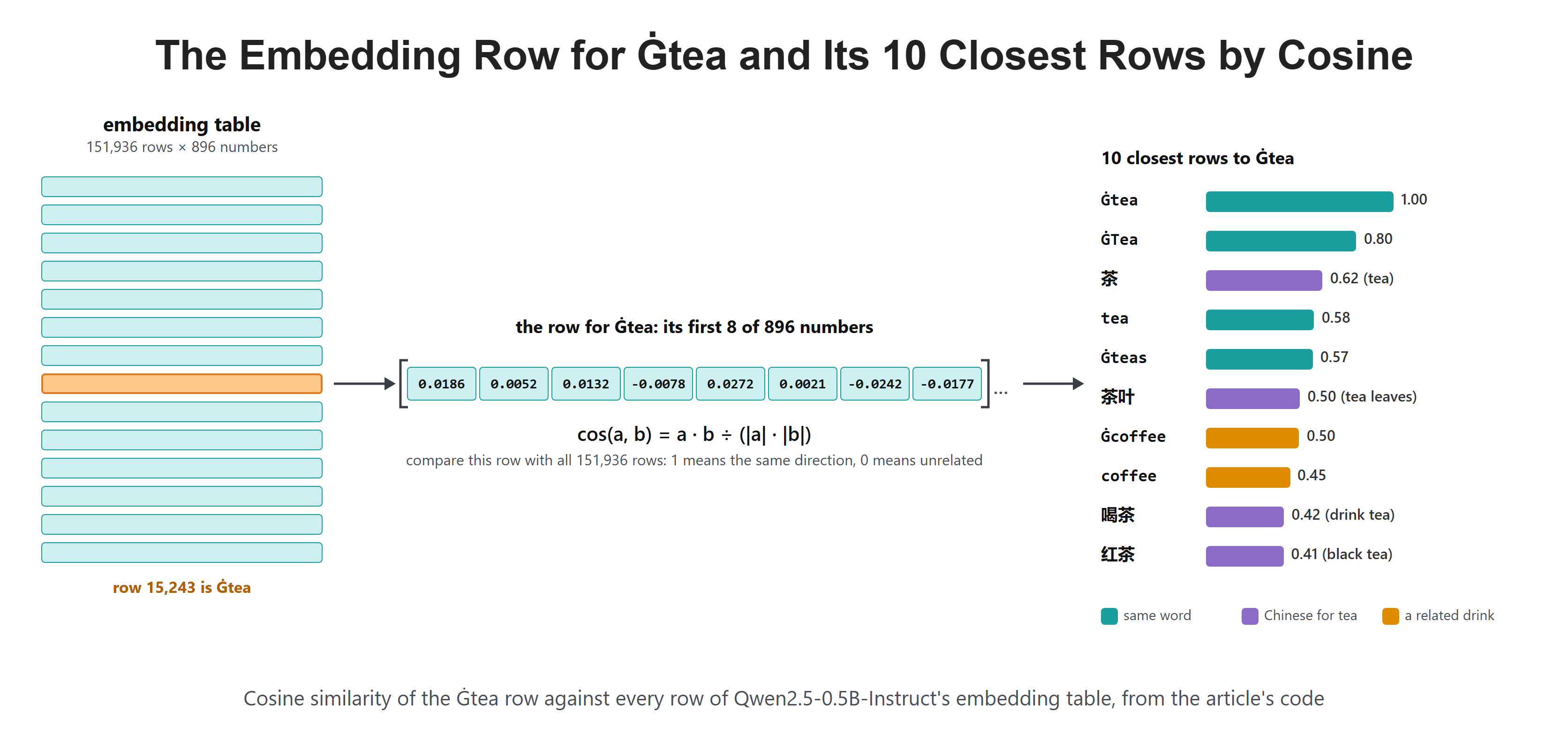
The figure below shows this lookup for Ġtea, which is row 15,243. On the right, it lists the 10 rows that point most nearly the same way as the Ġtea row. We will compute both with code.
First, let's check the shape of the table.
E = model.model.embed_tokens.weight.float()
E.shapetorch.Size([151936, 896])The table has 151,936 rows of 896 numbers each, which is 136,134,656 weights. That is more than a quarter of the whole model. It also has 271 more rows than the tokenizer has entries, so no token ever reads those last rows.
To see what the table has learned, we compare the row for Ġtea with every other row. Cosine similarity measures how closely two vectors point the same way:
Where:
- , : two rows of the embedding table
- : their dot product
- : the length of
- the result: 1 means the same direction, 0 means unrelated
Let's find the 10 closest rows to Ġtea.
tea = E[tok.encode(" tea")[0]]
similarity = torch.cosine_similarity(E, tea[None], dim=-1)
[tok.decode(i) for i in similarity.topk(10).indices.tolist()][' tea', ' Tea', '茶', 'tea', ' teas', '茶叶', ' coffee', 'coffee', '喝茶', '红茶']Here, we can see other forms of "tea", the Chinese words for tea, tea leaves, drinking tea and black tea, and coffee, a related drink. Nobody wrote these links. Training placed tokens that are used in similar ways close together.
What Happens Inside One Decoder Layer?
Every decoder layer does two jobs on a stream of vectors, one vector of 896 numbers per token. This stream is called the residual stream. First, attention lets each token collect information from the tokens before it. Then the MLP works on each token alone.
Each job reads a normalized copy of the stream and adds its result back:
Where:
- : the layer's input, one row of 896 numbers per token
- : the stream after the attention job
- : the layer's output, which is the next layer's input
- , : the modules
input_layernormandpost_attention_layernorm
In simple words, each layer edits the vectors and never replaces them. The added keeps what the token already knew. The norm runs only on the copy that goes into attention or the MLP, not on the stream itself. This order, norm first and add after, is called pre-norm. The original Transformer did it the other way round, adding first and normalizing after, which is the "Add & Norm" box in its figure.
What Does RMSNorm Do?
Vectors in the residual stream can grow or shrink from layer to layer. Attention and the MLP work best when their inputs have a steady size. So every layer first rescales its input with a norm.
The original Transformer uses LayerNorm. It subtracts the mean, divides by the standard deviation, then multiplies by a learned weight and adds a learned bias. Qwen2.5's RMSNorm keeps only the rescaling. It divides each vector by its root mean square and multiplies by a learned weight:
Where:
- : one token's vector
- : its length, 896 in Qwen2.5
- : a tiny number, 1e-6 in Qwen2.5, that keeps the division safe
- : the learned weight, one number per position in the vector
- : multiply position by position
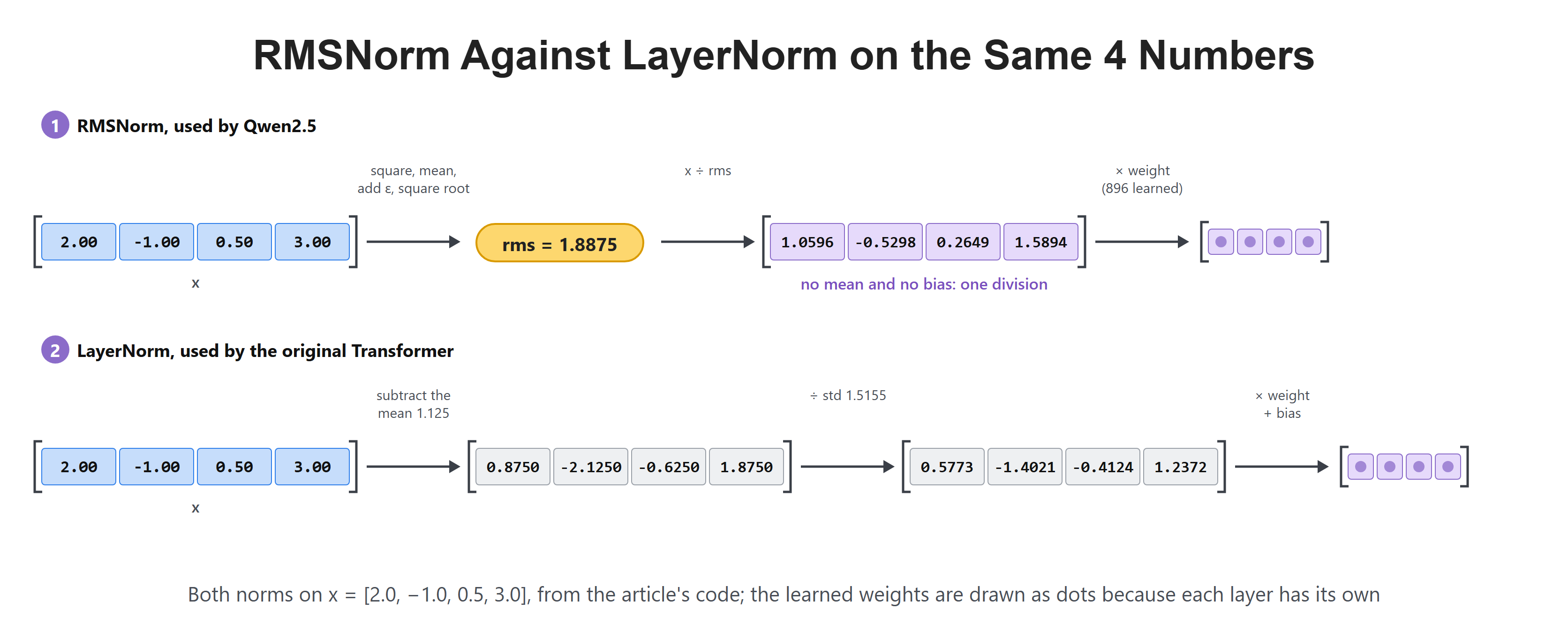
The figure below runs both norms on the same 4 numbers. RMSNorm divides by one number, the root mean square 1.8875. LayerNorm first subtracts the mean 1.125, then divides by the standard deviation 1.5155.
Let's try both norms on 4 numbers. First the RMSNorm division, without the learned weight:
x = torch.tensor([2.0, -1.0, 0.5, 3.0])
rms = x.pow(2).mean().add(1e-6).sqrt()
rms, x / rms(tensor(1.8875), tensor([ 1.0596, -0.5298, 0.2649, 1.5894]))Here, we can see that the root mean square is 1.8875, and every number is divided by it. The signs and the ratios between the numbers stay the same. Only the size changes.
Now LayerNorm on the same numbers:
torch.nn.functional.layer_norm(x, (4,))tensor([ 0.5773, -1.4021, -0.4124, 1.2372])LayerNorm first moves the mean to 0, so it gives a different result: 2.0 becomes 0.5773 instead of 1.0596.
Why Does a Token Need Attention?
So far, every token has its own vector, and that vector knows only its own token.
Let's read two sentences:
- The cat sat on the mat because it was tired.
- The trophy did not fit in the suitcase because it was too big.
In the first sentence, "it" means the cat. In the second, it means the trophy. But both "it" tokens get the same id, 432, so the embedding lookup hands them the same row. To find out what "it" means, the token must look at the other words in its sentence.
So, here comes attention to the rescue. Attention is the step that lets every token look at the tokens before it and pull in what it needs. Inside a decoder layer, it is the only part that mixes tokens. RMSNorm and the MLP work on each token alone.
The figure below follows the vector for "it" through the 24 layers, in both sentences.
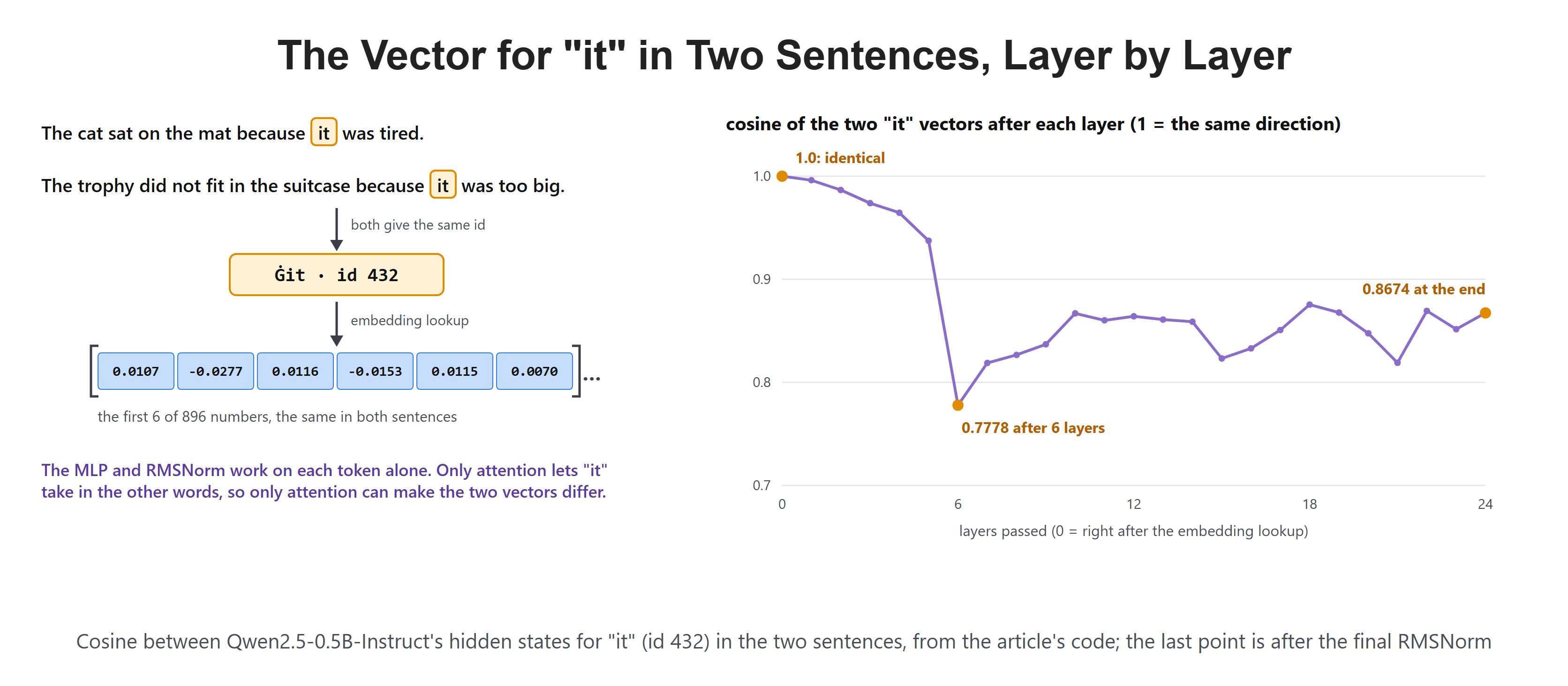
Here, we can see that the two vectors start identical and then drift apart. Let's measure this with code. hidden_states[0] is the vector right after the embedding lookup, and hidden_states[n] is the vector after n layers.
def vector_of_it(sentence, layer):
    x = tok(sentence, return_tensors="pt").to("cuda")
    hidden = model(**x, output_hidden_states=True).hidden_states[layer][0]
    tokens = tok.convert_ids_to_tokens(x["input_ids"][0])
    return hidden[tokens.index("Ġit")].float()

a = "The cat sat on the mat because it was tired."
b = "The trophy did not fit in the suitcase because it was too big."
[round(torch.cosine_similarity(vector_of_it(a, layer), vector_of_it(b, layer), dim=0).item(), 4) for layer in (0, 1, 6, 24)][1.0, 0.9961, 0.7778, 0.8674]The cosine starts at 1.0, because both vectors are the same row of the embedding table. After 1 layer it is 0.9961, after 6 layers 0.7778, and at the end 0.8674. The last value also includes the final RMSNorm. RMSNorm and the MLP alone would keep two identical vectors identical forever, so the drift comes from attention: each "it" took in different words.
How Does Self-Attention Work?
Self-attention is the kind of attention Qwen uses: every token looks at tokens of its own sequence. Before we look at Qwen's real heads, let's compute one attention head by hand, exactly as the notebook does. Let's say we have four tokens, It's, time, for and tea, each a vector of 8 numbers, and one head of size 4. The numbers are random, drawn with a fixed seed so that we get the same values every time.
Attention follows one formula:
Where:
- : the queries, what each token is looking for
- : the keys, what each token offers to be matched on
- : the values, what each token hands over
- : the head size, 4 here and 64 in Qwen2.5
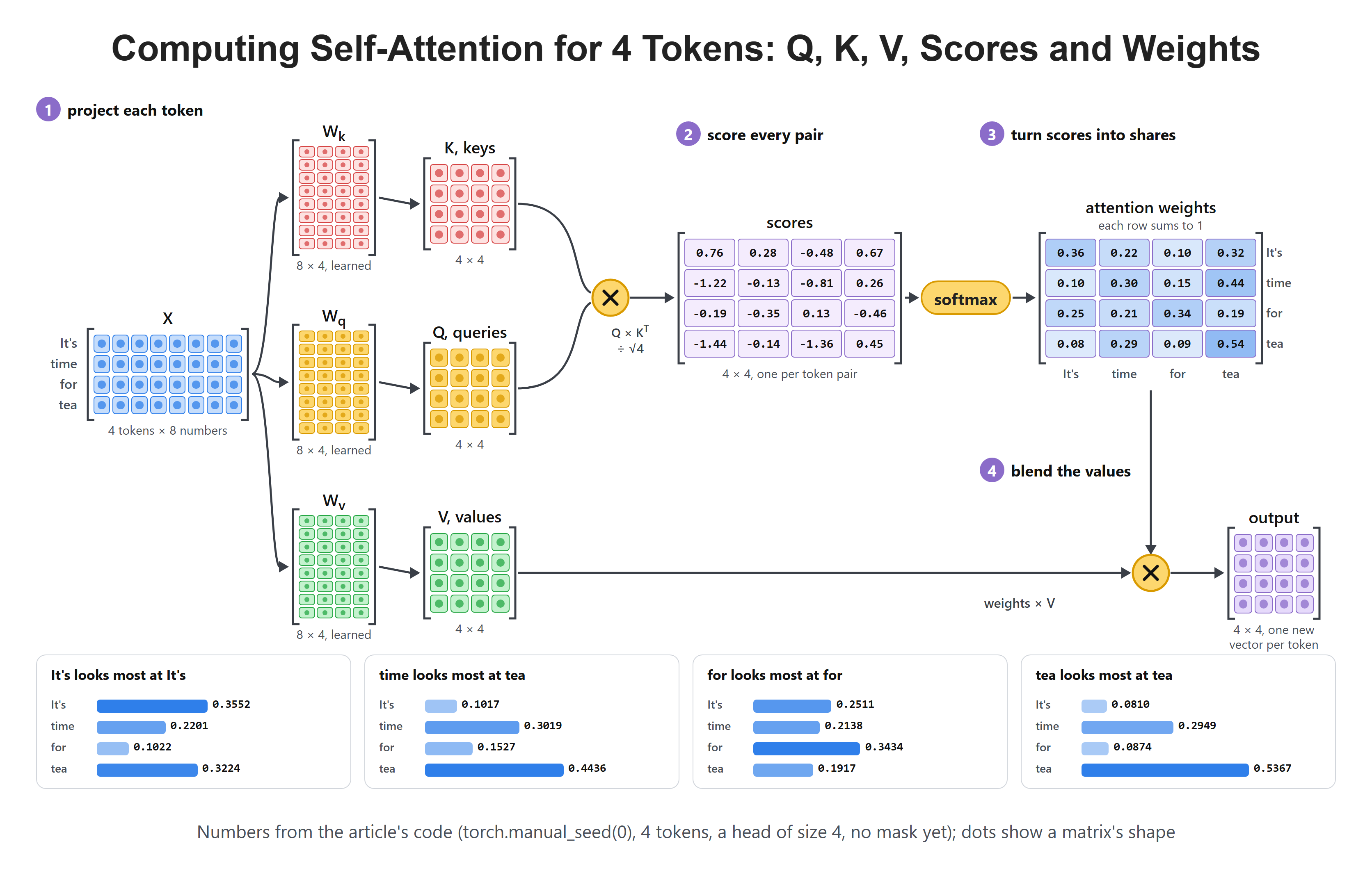
The figure below shows the whole computation for our 4 tokens in one picture. Each token is projected into a query, a key and a value. Every query is scored against every key, softmax turns each row of scores into weights, and the weights blend the values into one new vector per token. The cards at the bottom show where each token looks the most.
Now let's build it step by step. First, three weight matrices turn the token vectors into Q, K and V. The figure below shows the three projections with the real values our code will produce.
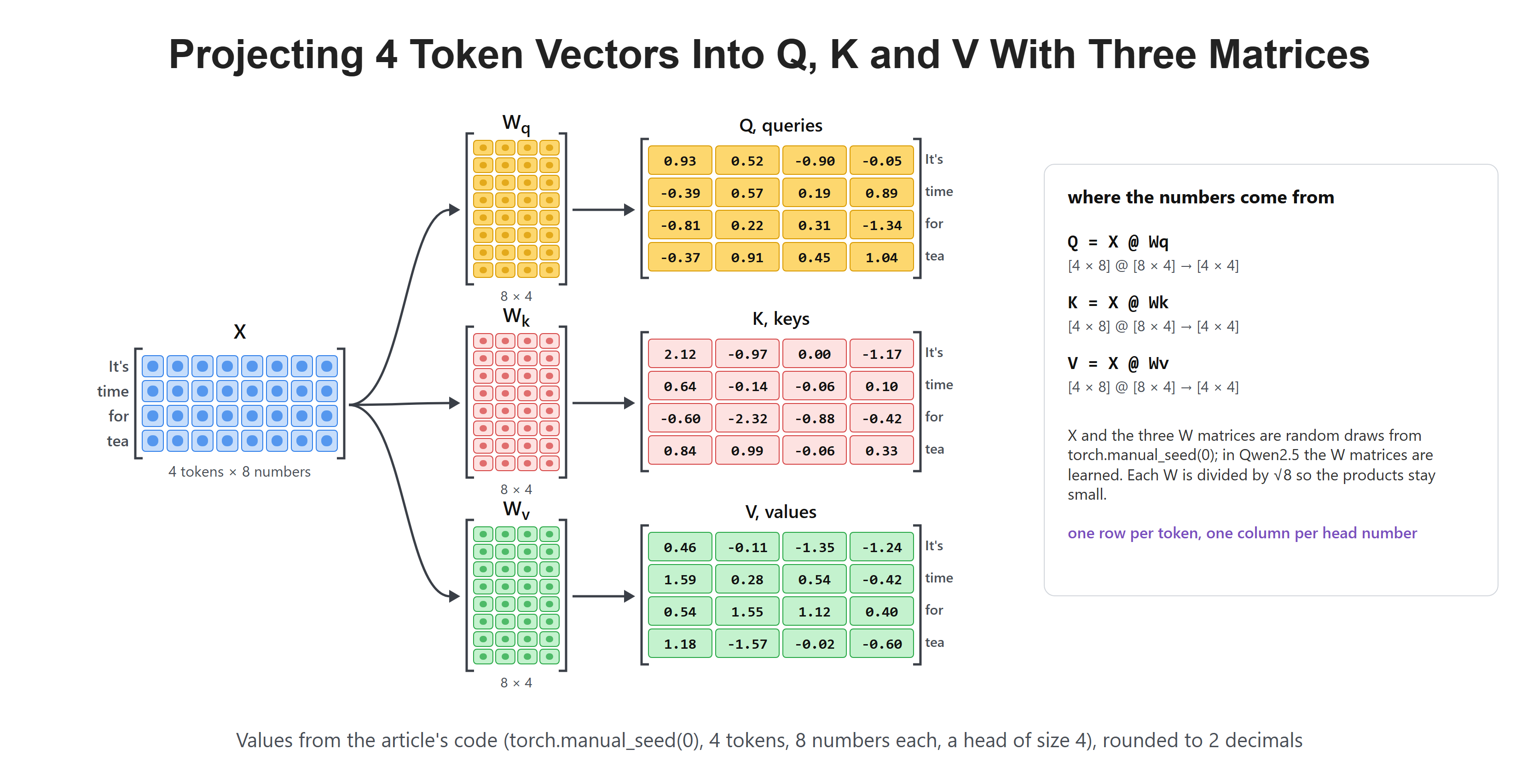
Let's see the code as below.
torch.manual_seed(0)
X = torch.randn(4, 8)
Wq = torch.randn(8, 4) / math.sqrt(8)
Wk = torch.randn(8, 4) / math.sqrt(8)
Wv = torch.randn(8, 4) / math.sqrt(8)

Q = X @ Wq
K = X @ Wk
V = X @ Wv
Q.shapetorch.Size([4, 4])Each of Q, K and V has one row per token and 4 numbers per row, the head size.
Next, every query is compared with every key, the scores are scaled by , and softmax turns each row into weights. The figure below shows these steps on our numbers: the raw scores, the scaling and the softmax. Its last grid adds the causal mask, which we will meet in a moment.
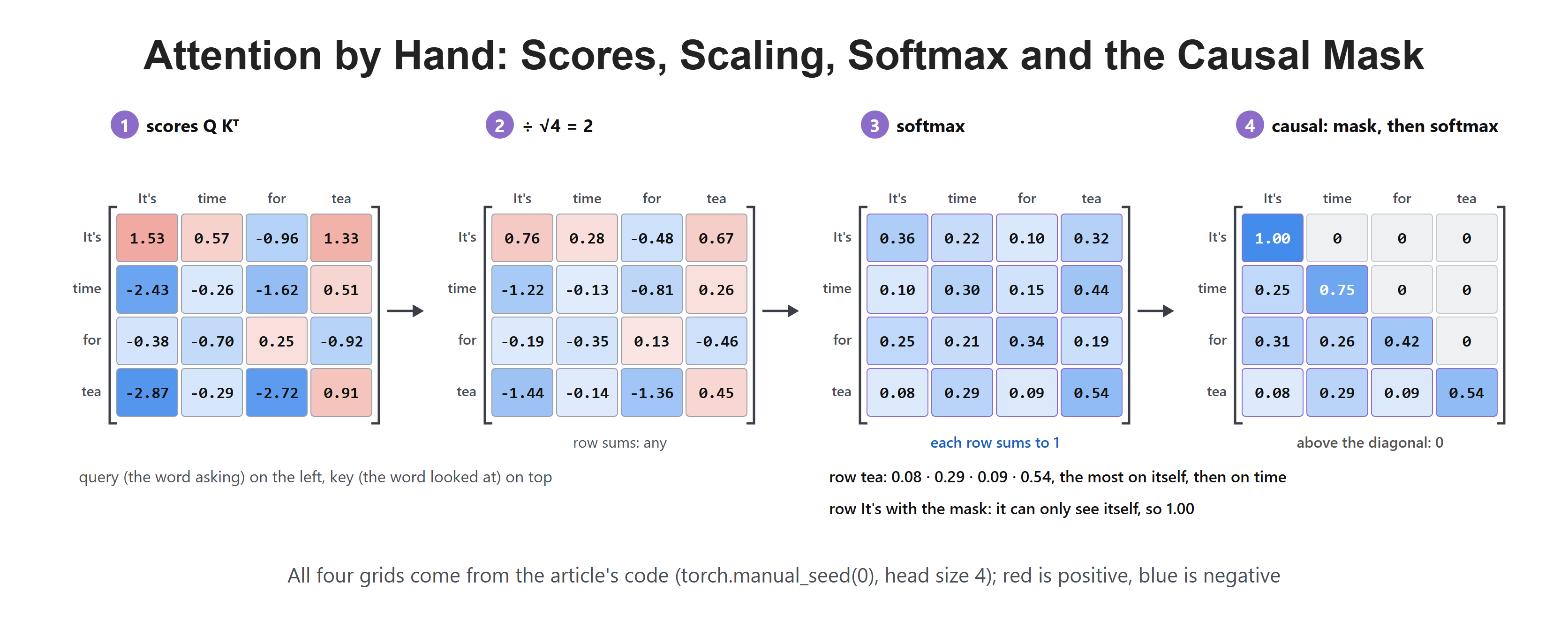
Let's see the code as below.
scores = (Q @ K.T) / math.sqrt(4)
weights = torch.softmax(scores, dim=-1)
weightstensor([[0.3552, 0.2201, 0.1022, 0.3224],
[0.1017, 0.3019, 0.1527, 0.4436],
[0.2511, 0.2138, 0.3434, 0.1917],
[0.0810, 0.2949, 0.0874, 0.5367]])Here, we can see a 4 × 4 grid of weights, one row per token. The row for tea puts 0.5367 on itself and 0.2949 on time. Let's check the row sums.
weights.sum(dim=-1)tensor([1., 1., 1., 1.])Every row sums to 1, because softmax turns each row of scores into shares. The output blends the value rows by these shares.
out = weights @ V
outtensor([[ 0.9502, -0.3241, -0.2500, -0.6852],
[ 1.1327, -0.3864, 0.1902, -0.4594],
[ 0.8674, 0.2653, 0.1599, -0.3794],
[ 1.1864, -0.6340, 0.1394, -0.5130]])Each output row is a new vector for its token, mixed from all four value rows.
The Causal Mask
A decoder writes left to right, so a token must never look at the tokens after it. A causal mask marks which pairs are allowed.
mask = torch.tril(torch.ones(4, 4)).bool()
masktensor([[ True, False, False, False],
[ True, True, False, False],
[ True, True, True, False],
[ True, True, True, True]])We set the blocked scores to minus infinity before softmax, so they become 0.
causal_weights = torch.softmax(scores.masked_fill(~mask, float("-inf")), dim=-1)
causal_weightstensor([[1.0000, 0.0000, 0.0000, 0.0000],
[0.2520, 0.7480, 0.0000, 0.0000],
[0.3107, 0.2645, 0.4249, 0.0000],
[0.0810, 0.2949, 0.0874, 0.5367]])Here, we can see that every weight above the diagonal is now 0. The row for It's can only see itself, so it gets 1.0. The row for tea could already see every token, so its weights do not change.
PyTorch has the same thing built in, as one fast function.
torch.nn.functional.scaled_dot_product_attention(Q, K, V, is_causal=True)tensor([[ 0.4644, -0.1060, -1.3465, -1.2355],
[ 1.3065, 0.1847, 0.0644, -0.6232],
[ 0.7935, 0.7012, 0.2017, -0.3259],
[ 1.1864, -0.6340, 0.1394, -0.5130]])Let's compare it with our own masked weights times V.
causal_weights @ Vtensor([[ 0.4644, -0.1060, -1.3465, -1.2355],
[ 1.3065, 0.1847, 0.0644, -0.6232],
[ 0.7935, 0.7012, 0.2017, -0.3259],
[ 1.1864, -0.6340, 0.1394, -0.5130]])The two results match exactly. In Qwen2.5, , and are the q_proj, k_proj and v_proj layers we saw in the model printout, and each head is 64 numbers wide instead of 4.
How Does Multi-Head Attention Work?
One head learns one way of matching queries to keys. But a sentence has many kinds of links at once: which noun a pronoun points to, which word came just before, where the sentence started. One head cannot follow all of them.
So, instead of one big head, we run several smaller heads side by side. Each head gets its own slice of Q, K and V and computes its own weights. Then we put the heads' outputs side by side, which is called concat, and one more matrix, the output projection, mixes them back into one vector per token. This is multi-head attention.
The figure below shows it on our 4 tokens with 2 heads of 4 numbers each. Each head has its own , and , makes its own Q, K and V, and computes its own causal weights. The results and are joined and mixed by .
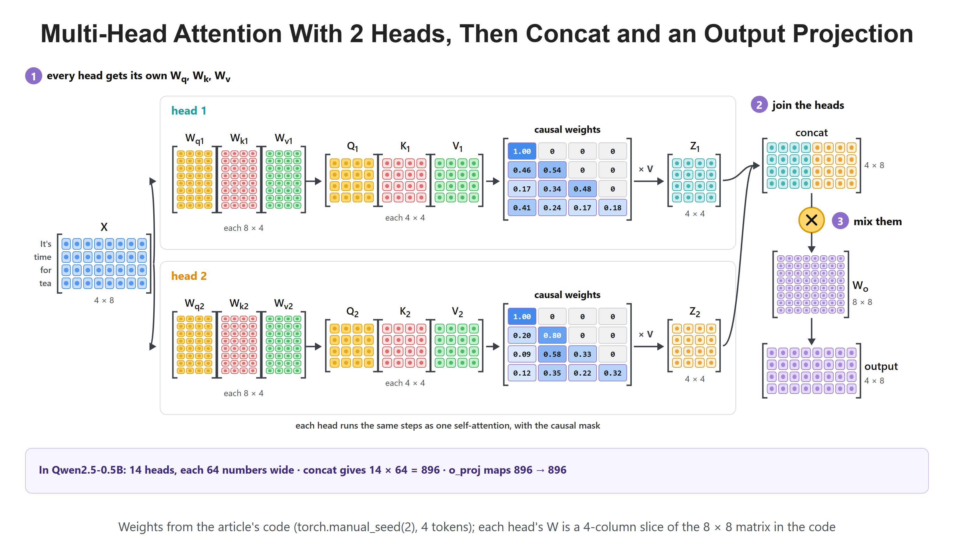
Let's see the code as below. split_heads cuts the 8 numbers of each token into 2 slices of 4, one per head. Splitting the output of one 8 × 8 matrix this way is the same as giving each head its own 8 × 4 matrix, as in the figure.
torch.manual_seed(2)
Wq2, Wk2, Wv2, Wo = (torch.randn(8, 8) / math.sqrt(8) for _ in range(4))

def split_heads(M):
    return M.view(4, 2, 4).transpose(0, 1)   # 4 tokens x 8 numbers -> 2 heads x 4 tokens x 4 numbers

Qh, Kh, Vh = split_heads(X @ Wq2), split_heads(X @ Wk2), split_heads(X @ Wv2)
scores_h = (Qh @ Kh.transpose(1, 2)) / math.sqrt(4)
weights_h = torch.softmax(scores_h.masked_fill(~mask, float("-inf")), dim=-1)
weights_htensor([[[1.0000, 0.0000, 0.0000, 0.0000],
[0.4558, 0.5442, 0.0000, 0.0000],
[0.1749, 0.3447, 0.4804, 0.0000],
[0.4130, 0.2355, 0.1679, 0.1836]],
[[1.0000, 0.0000, 0.0000, 0.0000],
[0.2029, 0.7971, 0.0000, 0.0000],
[0.0893, 0.5781, 0.3326, 0.0000],
[0.1151, 0.3511, 0.2171, 0.3167]]])Here, we can see two grids of weights, one per head, and the causal mask holds in both. The two heads read the same tokens but weigh them differently. The row for tea puts the most, 0.4130, on It's in head 1, and the most, 0.3511, on time in head 2.
Now each head blends its own values. Then we concat the heads and apply the output projection.
heads_out = weights_h @ Vh
concat = heads_out.transpose(0, 1).reshape(4, 8)
out = concat @ Wo
heads_out.shape, concat.shape, out.shape(torch.Size([2, 4, 4]), torch.Size([4, 8]), torch.Size([4, 8]))Each head gives 4 numbers per token. Concat puts the two heads side by side, 8 numbers per token, and mixes them into the output, still 4 tokens × 8 numbers.
Qwen2.5 does the same at full size. It runs 14 heads in every layer, each 64 numbers wide, and 14 × 64 = 896. Splitting is only a reshape of the same numbers.
x = torch.randn(5, 896)
heads = x.view(5, 14, 64)
heads.shapetorch.Size([5, 14, 64])Here, 5 token vectors of 896 numbers become 5 tokens × 14 heads × 64 numbers. Qwen's output projection is o_proj.
model.model.layers[0].self_attn.o_proj.weight.shapetorch.Size([896, 896])It takes the 896 concatenated numbers and maps them back to 896, one vector per token, ready to be added to the residual stream.
Why Does Qwen Use Grouped-Query Attention?
While a model generates text, it saves the keys and values of every token it has already read, so that it does not compute them again on every step. This saved memory is called the KV cache. In the multi-head attention we just built, every query head has its own key head and value head. With 14 heads, the cache grows quickly with every token.
So, here comes grouped-query attention to the rescue. The query heads are split into groups, and each group shares one key head and one value head. The figure below shows how Qwen2.5 does this.
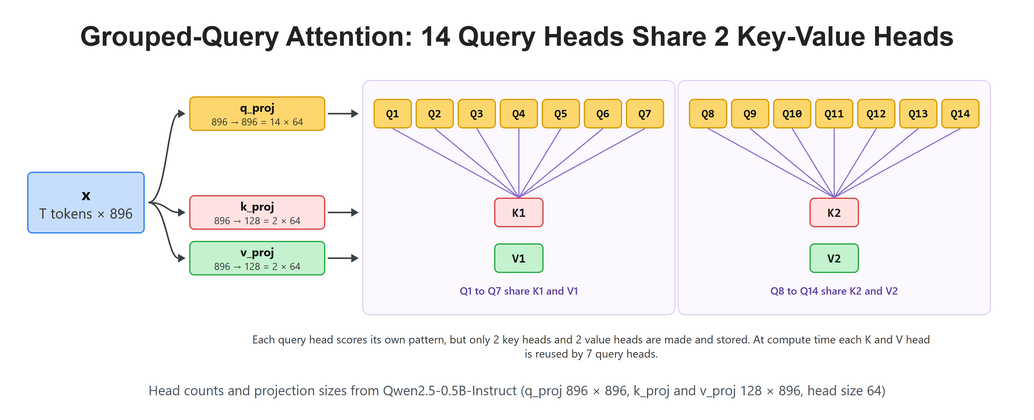
Query heads 1 to 7 read key head 1 and value head 1. Query heads 8 to 14 read key head 2 and value head 2. Each query head still has its own query weights, so it can still look for its own pattern. Only the keys and values are shared.
Let's look at the projection shapes in the first layer.
attn = model.model.layers[0].self_attn
attn.q_proj.weight.shape, attn.k_proj.weight.shape, attn.v_proj.weight.shape(torch.Size([896, 896]), torch.Size([128, 896]), torch.Size([128, 896]))Here, we can see that q_proj makes 896 numbers, 14 heads of 64. But k_proj and v_proj make only 128 numbers each, which is 2 heads of 64.
Attention still needs one key head for every query head when it computes the scores. So before attention runs, Qwen copies each key head and value head 7 times with a function called repeat_kv. Let's try it on random keys for 5 tokens.
from transformers.models.qwen2.modeling_qwen2 import repeat_kv

k = torch.randn(1, 2, 5, 64)   # 1 sentence, 2 key heads, 5 tokens, 64 numbers
shared = repeat_kv(k, 7)
shared.shape, torch.equal(shared[0, 0], shared[0, 6]), torch.equal(shared[0, 7], k[0, 1])(torch.Size([1, 14, 5, 64]), True, True)Here, the 2 key heads become 14. Heads 0 to 6 are all copies of the first key head, so heads 0 and 6 hold the same numbers. Head 7 is a copy of the second key head. These copies exist only while attention runs. The KV cache stores just the 2 real heads.
Now let's measure what this saves. The cache stores one key and one value per layer, per KV head and per token, at 2 bytes per bfloat16 number. The figure below multiplies this out for one token and for a full 32,768-token context.
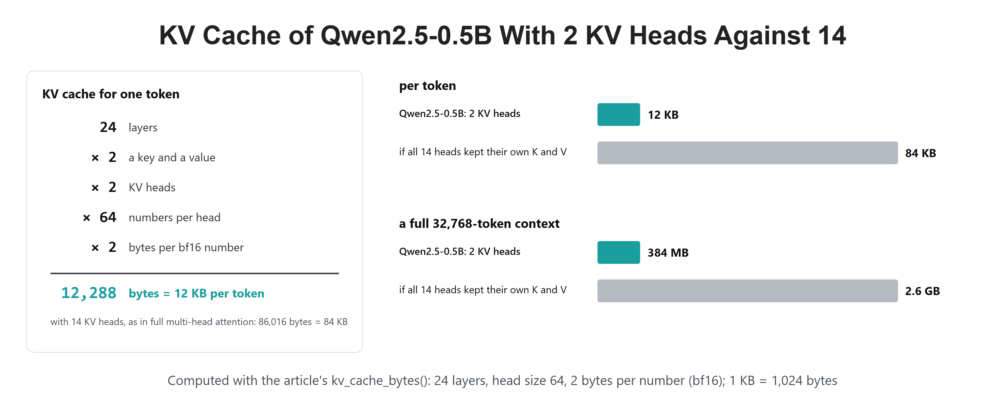
Let's compute it in code.
def kv_cache_bytes(kv_heads, tokens, layers=24, head_dim=64, bytes_per_number=2):
    return layers * 2 * kv_heads * head_dim * bytes_per_number * tokens

kv_cache_bytes(2, 1), kv_cache_bytes(14, 1)(12288, 86016)Here, one token needs 12,288 bytes of cache, which is 12 KB. If every query head kept its own key and value head, one token would need 86,016 bytes, which is 84 KB. That is 7 times more. Let's scale this up to the full context.
kv_cache_bytes(2, 32768) / 1024**2, kv_cache_bytes(14, 32768) / 1024**3(384.0, 2.625)At the full 32,768-token context, the cache needs 384 MB with grouped-query attention. Without it, the same context would need 2.625 GB.
What Is Cross-Attention, and Why Does Qwen Not Use It?
So far, every token has looked at tokens of its own sequence. Cross-attention is the version where one sequence looks at another. It is the middle attention block in the decoder of the original Transformer, the one that reads from the encoder.
Encoder-decoder models such as T5 use it for tasks like translation. The encoder reads the whole input first. Then, while the decoder writes, its queries come from the tokens it has written so far, and its keys and values come from the encoder's output. So every word being written can look back at the full input.
The figure below shows the whole computation on a small example. The steps are the same as in self-attention. Only the sources of Q, K and V differ.
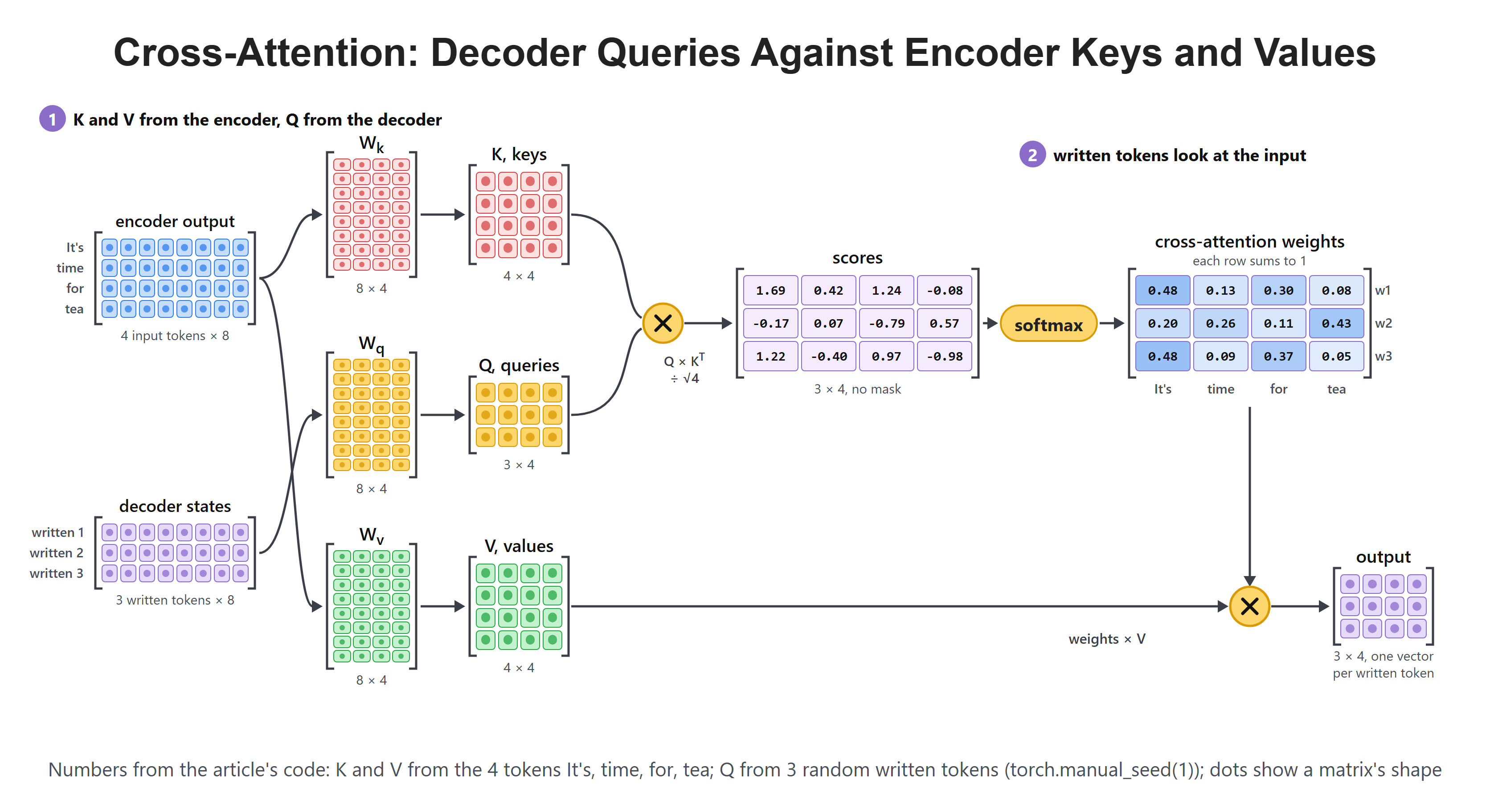
Let's compute it. Our 4 tokens, It's, time, for and tea, play the encoder's output, so we reuse their keys K and values V. Three new random vectors play the tokens the decoder has written.
torch.manual_seed(1)
Y = torch.randn(3, 8)   # 3 tokens the decoder has written so far

cross_weights = torch.softmax((Y @ Wq) @ K.T / math.sqrt(4), dim=-1)
cross_weightstensor([[0.4799, 0.1341, 0.3048, 0.0812],
[0.2048, 0.2600, 0.1096, 0.4255],
[0.4792, 0.0945, 0.3730, 0.0533]])Here, we can see a 3 × 4 grid: one row per written token and one column per input token. There is no causal mask, because the whole input already exists. Each row still sums to 1, and blending the values gives one output row per written token.
(cross_weights @ V).shapetorch.Size([3, 4])Qwen2.5 has no encoder, so it has nothing to cross-attend to. Instead, a decoder-only model puts the prompt and its answer into one sequence. With the causal mask, every answer token can look at all the prompt tokens, which is the job cross-attention does in an encoder-decoder model. The figure below marks these cells.
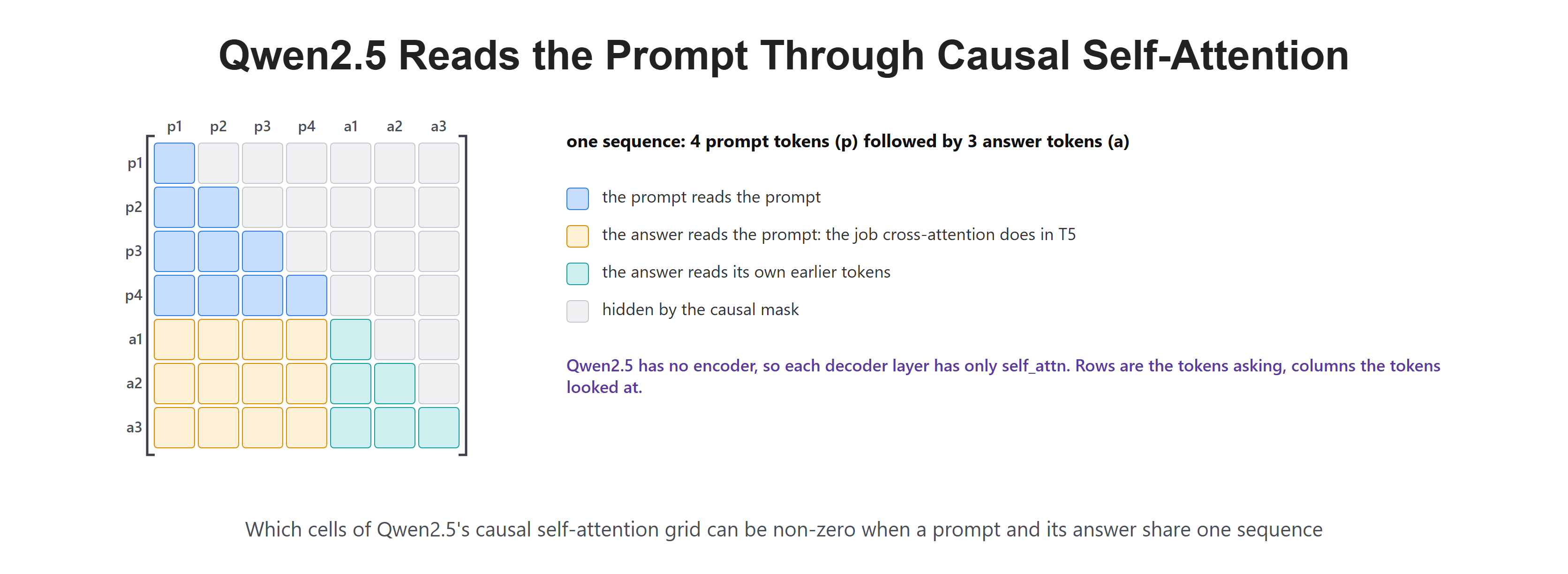
Let's confirm it in code by listing the parts of one decoder layer.
[name for name, _ in model.model.layers[0].named_children()]['self_attn', 'mlp', 'input_layernorm', 'post_attention_layernorm']Here, we can see only self_attn. There is no cross-attention module in Qwen2.5.
How Does RoPE Tell Positions Apart?
Attention compares vectors, and on its own it does not know the order of the tokens. "dog bites man" and "man bites dog" have the same three tokens. The original Transformer fixes this by adding a position vector to every token at the bottom of the model, the "Positional Encoding" in its figure. Qwen2.5 adds nothing at the bottom.
The figure below puts the two ideas side by side for "dog" in our two sentences. On the left, the original Transformer adds a different sin and cos vector to the same embedding. On the right, Qwen2.5 keeps the embedding as it is and turns the query and key of "dog" by an angle that depends on its position.
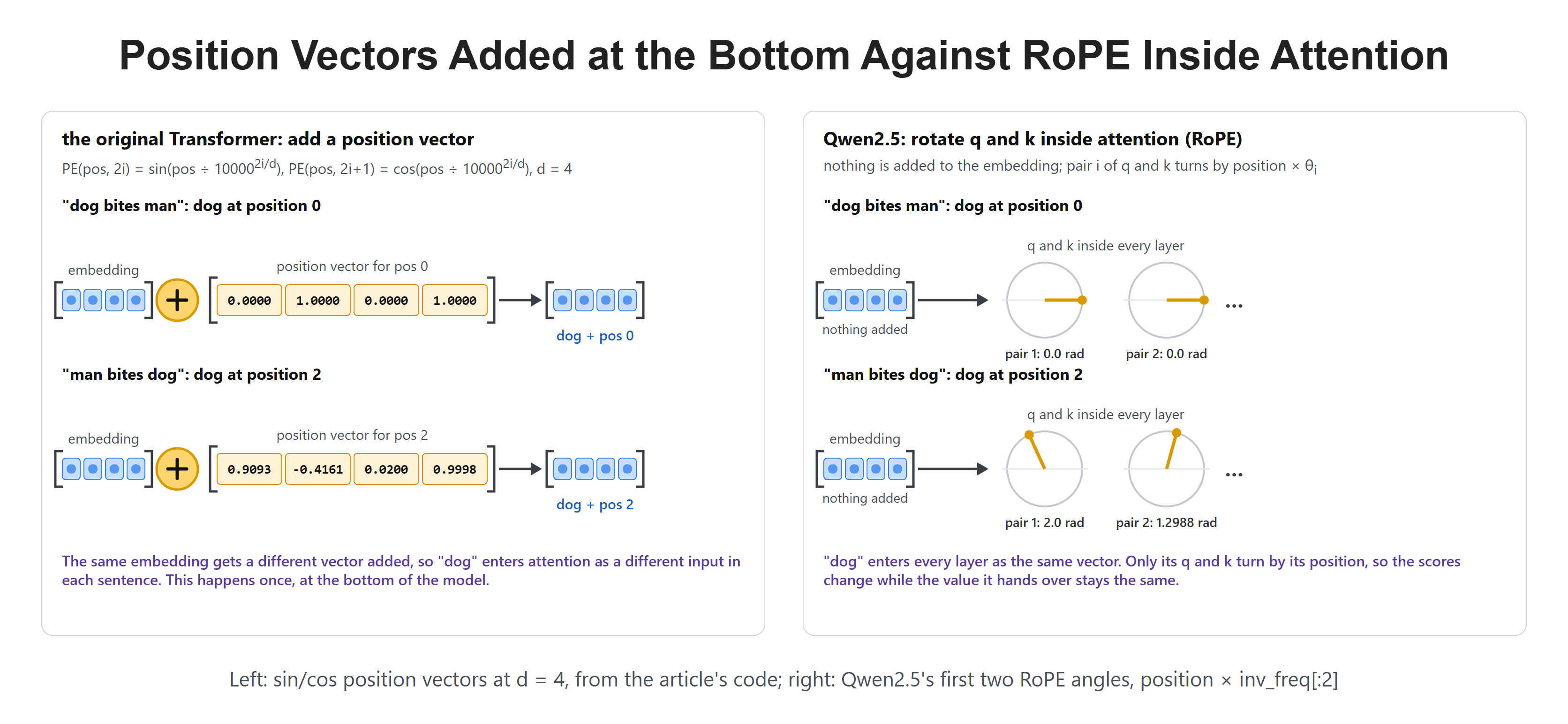
Let's compute the position vectors on the left, at d = 4. Even entries use sin and odd entries use cos.
def sinusoidal_position(position, d=4):
    i = torch.arange(0, d, 2)
    angle = position / 10000 ** (i / d)
    return torch.stack([angle.sin(), angle.cos()], dim=-1).flatten()

torch.stack([sinusoidal_position(p) for p in range(3)])tensor([[ 0.0000, 1.0000, 0.0000, 1.0000],
[ 0.8415, 0.5403, 0.0100, 0.9999],
[ 0.9093, -0.4161, 0.0200, 0.9998]])Here, we can see one fixed vector per position. Position 0 gets [0, 1, 0, 1], and position 2 gets a different vector, so the same embedding enters attention as a different input.
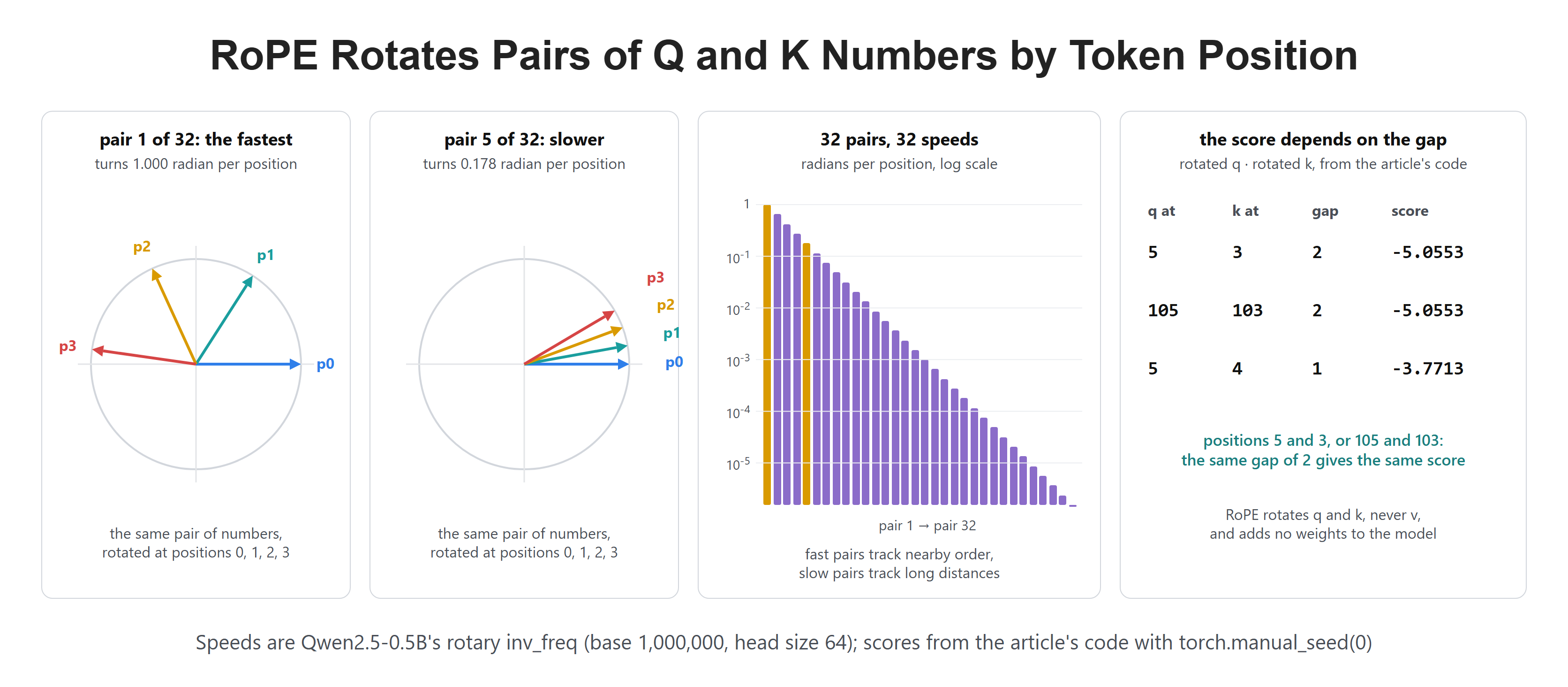
Instead, it uses RoPE, rotary position embedding. In simple words, RoPE takes the 64 numbers of every query head and every key head, treats them as 32 pairs, and rotates each pair by an angle that grows with the token's position. Each pair turns at its own speed:
Where:
- : how many radians pair turns per position
- : the RoPE base from Qwen2.5's config
- : the head size
- a token at position has pair turned by radians
The figure below shows RoPE on real numbers. The first two panels turn one pair at positions 0 to 3: the fastest pair and a slower one. The third panel shows all 32 speeds. The last panel shows the check that we will run at the end of this section.
The model stores these 32 speeds as inv_freq.
inv_freq = model.model.rotary_emb.inv_freq
inv_freq.shape, inv_freq[0].item(), inv_freq[-1].item()(torch.Size([32]), 1.0, 1.5399265294036013e-06)Here, we can see 32 speeds. The fastest pair turns 1 radian per position. The slowest turns about 0.0000015 radian per position, so it needs about 4 million positions to go around once. Fast pairs tell nearby tokens apart, and slow pairs still change over long distances.
Now the right half of the figure. The angle of pair is the position times $ heta_i$. Let's compute it for the first two pairs at positions 0 and 2.
torch.outer(torch.tensor([0.0, 2.0], device="cuda"), inv_freq[:2])tensor([[0.0000, 0.0000],
[2.0000, 1.2988]], device='cuda:0')
5 3 -5.0553
105 103 -5.0553
5 4 -3.7713At position 0, nothing turns. At position 2, pair 1 turns 2 radians and pair 2 turns 1.2988 radians, the two dials in the figure.
Why rotate? If we turn a query by one angle and a key by another, their dot product depends only on the difference between the two angles. So the score between a query at position and a key at position depends on , the distance between the two tokens. Let's test this with the model's own rotation code.
from transformers.models.qwen2.modeling_qwen2 import apply_rotary_pos_emb

def rotate(v, position):
    cos, sin = model.model.rotary_emb(v, torch.tensor([[position]], device="cuda"))
    return apply_rotary_pos_emb(v, v, cos, sin)[0]

torch.manual_seed(0)
q = torch.randn(1, 1, 1, 64, device="cuda")
k = torch.randn(1, 1, 1, 64, device="cuda")

for q_pos, k_pos in [(5, 3), (105, 103), (5, 4)]:
    score = (rotate(q, q_pos) * rotate(k, k_pos)).sum().item()
print(q_pos, k_pos, round(score, 4))5 3 -5.0553
105 103 -5.0553
5 4 -3.7713Here, we can see that positions 5 and 3 give the same score as positions 105 and 103, -5.0553, because both pairs are 2 positions apart. A gap of 1 gives a different score.
RoPE touches only the queries and keys, never the values. And inv_freq is a fixed buffer, not a learned weight, so RoPE adds no parameters to the model.
What Do Real Attention Heads Look At?
Now let's look at real heads. Qwen2.5-0.5B has 24 layers × 14 heads = 336 heads. The figure below shows four of them on the sentence "The cat sat on the mat because it was tired." Each row is one token, and it shows where that token looks. Darker cells mean more attention.
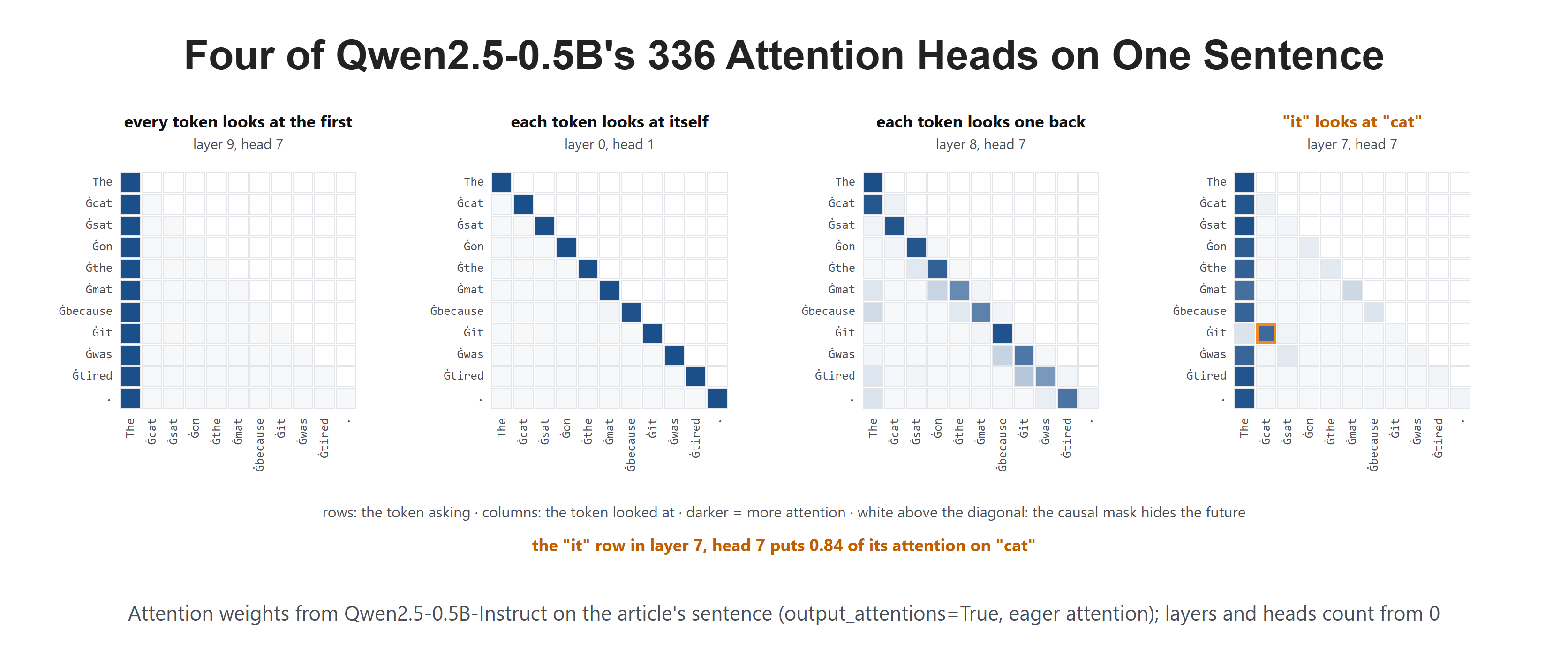
Training found these patterns, and nobody programmed them. Some heads look at the first token, some at the token itself, some one step back, and a few follow meaning, like "it" to "cat".
To get these weights ourselves, we need one change. The default attention code in transformers is fast but does not return its weights, so we switch to the eager version, which does.
model.set_attn_implementation("eager")

x = tok("The cat sat on the mat because it was tired.", return_tensors="pt").to("cuda")
response = model(**x, output_attentions=True)
len(response.attentions), response.attentions[0].shape(24, torch.Size([1, 14, 11, 11]))Here, we get one grid per layer: 14 heads, each with 11 tokens looking at 11 tokens. Let's ask one head where the token "it" looks.
tokens = tok.convert_ids_to_tokens(x["input_ids"][0])
A = response.attentions[7][0, 7].float().cpu()
tokens[7], tokens[A[7].argmax()], round(A[7].max().item(), 2)('Ġit', 'Ġcat', 0.84)In layer 7, head 7, the row for "it" puts 0.84 of its attention on "cat", the noun it refers to. Layers and heads count from 0 here. This is the fourth grid in the figure above.
Now let's ask the same head about the trophy sentence from the start of the attention part.
x = tok("The trophy did not fit in the suitcase because it was too big.", return_tensors="pt").to("cuda")
tokens = tok.convert_ids_to_tokens(x["input_ids"][0])
A = model(**x, output_attentions=True).attentions[7][0, 7].float().cpu()
tokens[9], tokens[A[9].argmax()], round(A[9].max().item(), 2)('Ġit', 'Ġtrophy', 0.51)Here, the same head sends 0.51 of the attention of "it" to "trophy", the noun it refers to. This is the kind of link that the embedding lookup alone could not give us.
Note
We keep eager attention on for the rest of this blog, as the course notebook does. The default attention code runs different GPU kernels, so its bfloat16 rounding moves the probabilities slightly: Ġthe below gets 0.2315 with it instead of 0.2259. The generated text stays the same.
What Does the SwiGLU MLP Do?
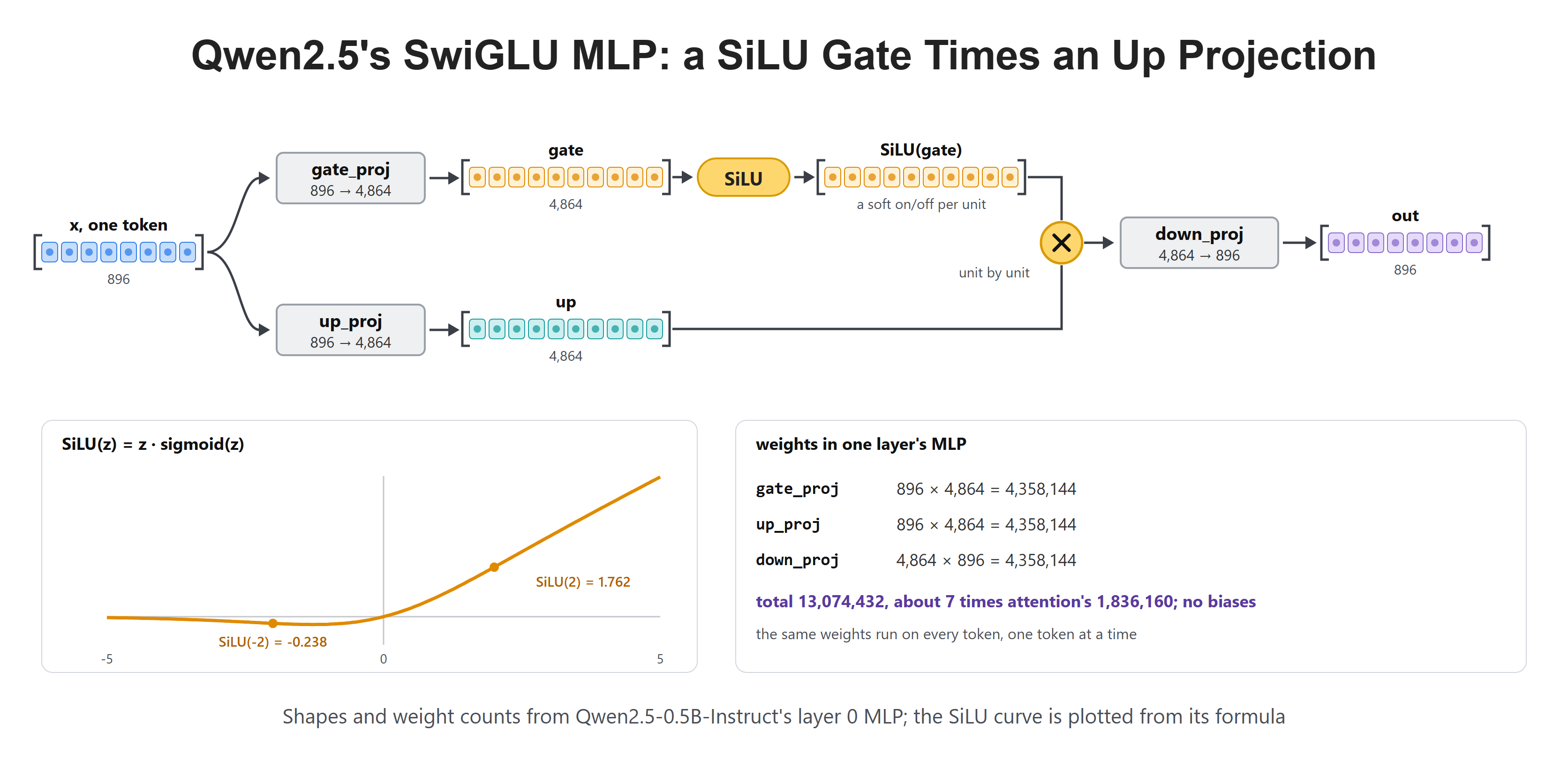
After attention has moved information between tokens, the MLP works on each token alone. The original Transformer's MLP, the "Feed Forward" box in its figure, widens the vector, applies ReLU and shrinks it back. Qwen2.5 uses SwiGLU, which adds a gate:
Where:
- : one token's 896 numbers
- , : the
gate_projandup_projmatrices, 896 → 4,864 - : the
down_projmatrix, 4,864 → 896 - : the sigmoid function
- : multiply unit by unit
In simple words, up_proj widens the token into 4,864 numbers. gate_proj makes a second set of 4,864 numbers and passes them through SiLU, which works like a soft on/off switch: large positive values pass, and negative values are pushed close to 0. Multiplying the two sets lets each of the 4,864 units be turned up or down by its own gate. Then down_proj squeezes the result back to 896 numbers.
The figure below shows this path for one token, the SiLU curve and the weight count of each matrix.
Let's count the weights in one layer's MLP and attention.
mlp = sum(p.numel() for p in model.model.layers[0].mlp.parameters())
attention = sum(p.numel() for p in model.model.layers[0].self_attn.parameters())
mlp, attention(13074432, 1836160)Here, the MLP holds 13,074,432 weights per layer, about 7 times attention's 1,836,160. That is three matrices of 896 × 4,864, with no biases.
Where Do the 494M Parameters Sit?
Now we can add up the whole model. The figure below shows where all 494,032,768 weights sit: in the 24 MLPs, the 24 attention blocks and the embedding table, which is also the LM head.
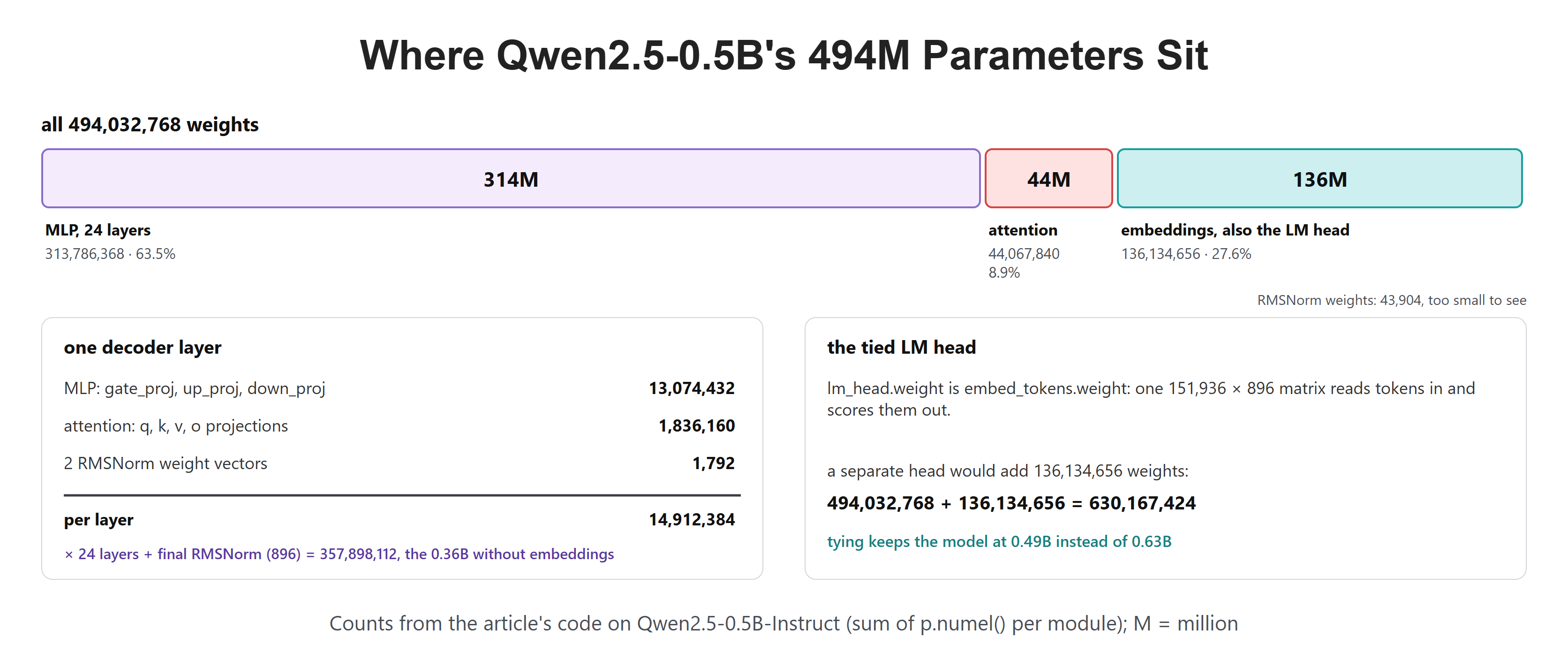
Let's check these numbers with code.
embeddings = model.model.embed_tokens.weight.numel()
total = sum(p.numel() for p in model.parameters())
embeddings, 24 * mlp, 24 * attention, total(136134656, 313786368, 44067840, 494032768)Here, the 24 MLPs hold 313,786,368 weights and the 24 attention blocks hold 44,067,840. The embedding table holds 136,134,656. Together with 43,904 RMSNorm weights, they add up to exactly 494,032,768.
The LM head does not appear in this sum as a separate matrix. Let's check why.
model.lm_head.weight is model.model.embed_tokens.weightTrueThe LM head is the embedding table itself. The same 151,936 × 896 matrix reads tokens in at the bottom and scores them at the top. A separate head would add another 136,134,656 weights.
How Do Logits Become the Next Token?
After the last layer and the final RMSNorm, the LM head turns each token's vector into 151,936 raw scores, one per vocabulary row. These scores are called logits.
The figure below follows the last token's vector through the LM head and softmax for two prompts. After the short prompt "It's time for", Ġtea is not in the top 5. After a longer prompt about a kettle, it leads.
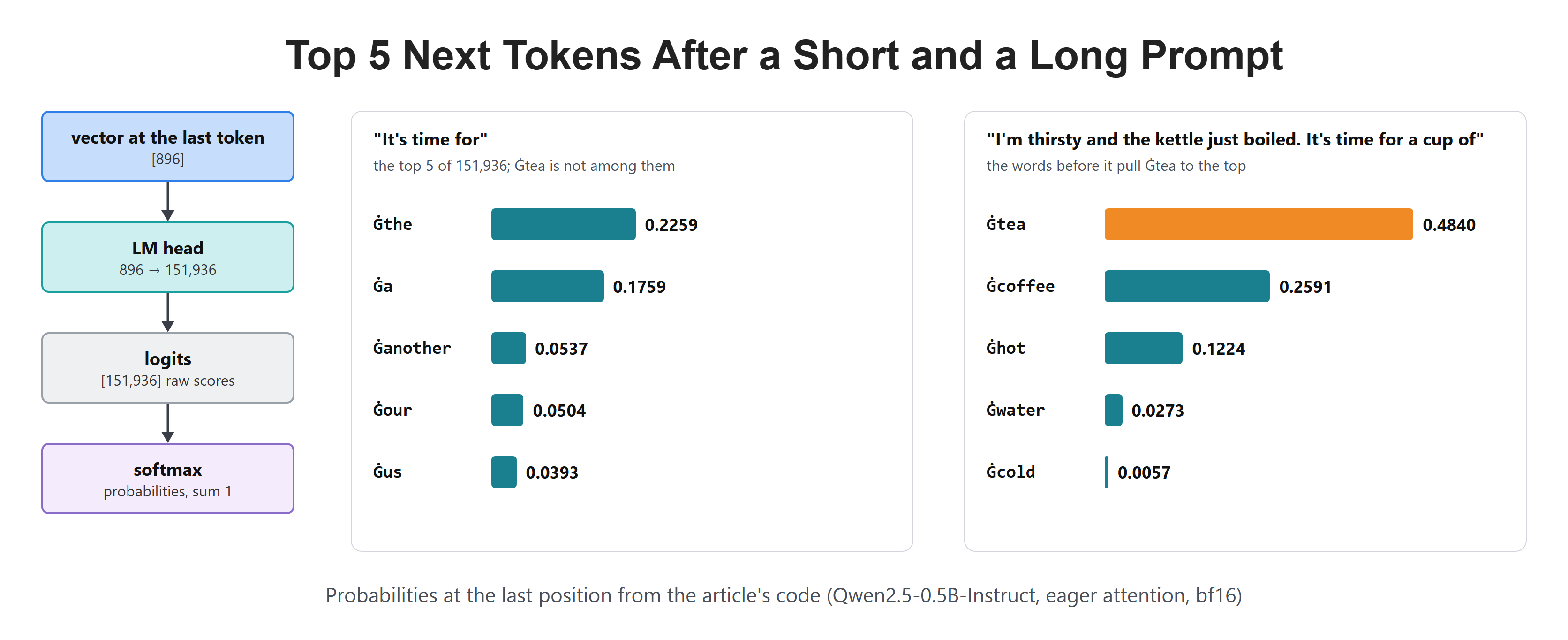
Let's start with the short prompt.
x = tok("It's time for", return_tensors="pt").to("cuda")
logits = model(**x).logits
logits.shapetorch.Size([1, 4, 151936])Here, we get one row of 151,936 logits for each of the 4 input tokens. Only the last row is used to pick the next token. Softmax turns it into probabilities that sum to 1.
probs = logits[0, -1].float().softmax(dim=-1)
top = probs.topk(5)
tok.convert_ids_to_tokens(top.indices), top.values(['Ġthe', 'Ġa', 'Ġanother', 'Ġour', 'Ġus'], tensor([0.2259, 0.1759, 0.0537, 0.0504, 0.0393], device='cuda:0'))After "It's time for", the model spreads its bets. Ġthe gets 0.2259 and Ġa gets 0.1759, and Ġtea is not in the top 5.
Context Changes the Scores
Now let's keep the same last words but give the model more context before them.
x = tok("I'm thirsty and the kettle just boiled. It's time for a cup of", return_tensors="pt").to("cuda")
probs = model(**x).logits[0, -1].float().softmax(dim=-1)
top = probs.topk(5)
tok.convert_ids_to_tokens(top.indices), top.values(['Ġtea', 'Ġcoffee', 'Ġhot', 'Ġwater', 'Ġcold'], tensor([0.4840, 0.2591, 0.1224, 0.0273, 0.0057], device='cuda:0'))Now Ġtea leads with 0.4840. Attention carried "thirsty" and "kettle" forward to the last position, and that changed the scores.
How Does Generation Work?
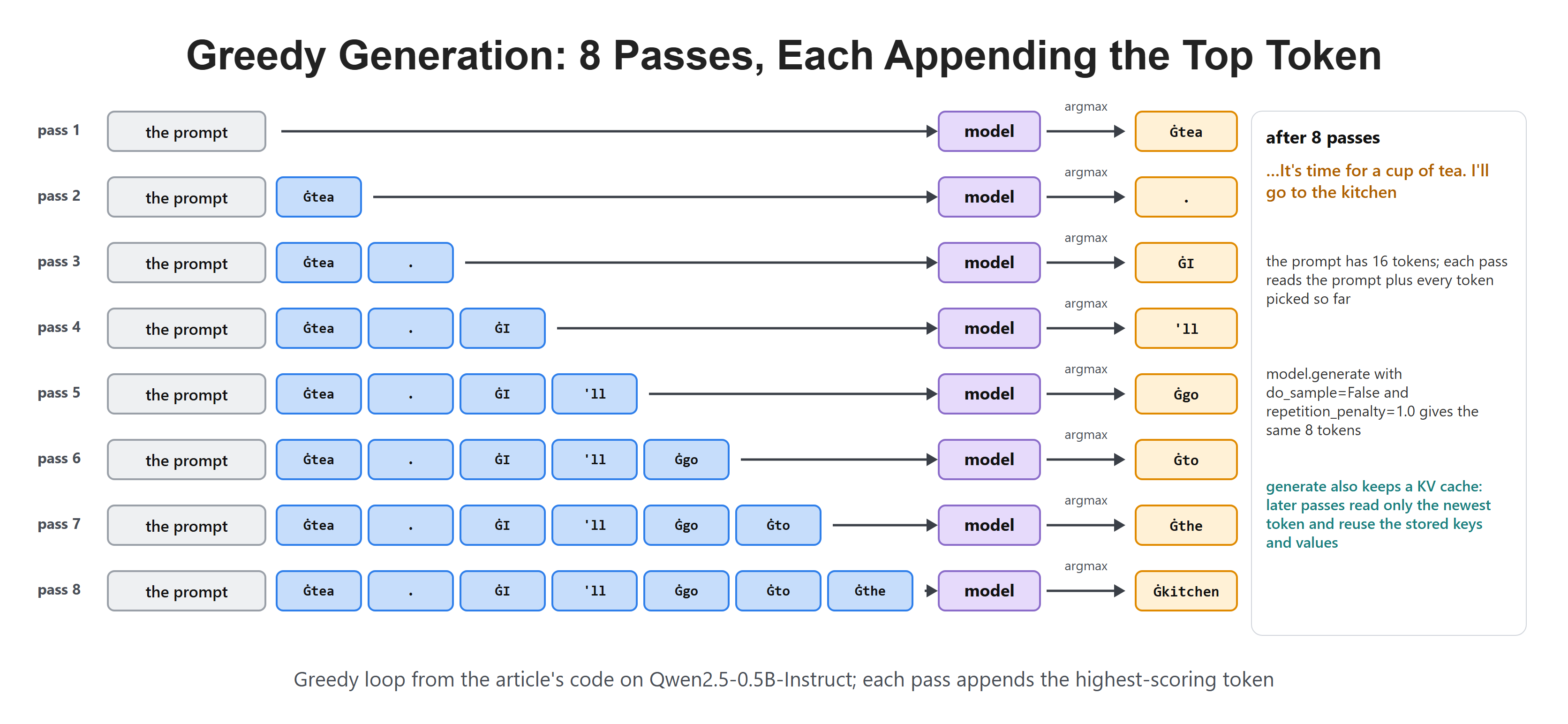
Generation is a loop. We take the top token, append it to the input and run the model again. Always taking the top token is called greedy decoding.
The figure below shows 8 such passes on our kettle prompt. Each pass reads the prompt plus every token picked so far, and appends one more.
Let's write this loop ourselves.
ids = tok("I'm thirsty and the kettle just boiled. It's time for a cup of", return_tensors="pt").to("cuda")["input_ids"]

for _ in range(8):
    next_id = model(ids).logits[0, -1].argmax()
    ids = torch.cat([ids, next_id.view(1, 1)], dim=1)

tok.decode(ids[0])"I'm thirsty and the kettle just boiled. It's time for a cup of tea. I'll go to the kitchen"Here, eight passes added "tea. I'll go to the kitchen", one token per pass. Hugging Face's generate runs the same loop. Qwen's saved generation settings turn on sampling and a repetition penalty of 1.1, so we switch both off to get greedy decoding.
x = tok("I'm thirsty and the kettle just boiled. It's time for a cup of", return_tensors="pt").to("cuda")
response = model.generate(**x, max_new_tokens=8, do_sample=False, repetition_penalty=1.0)
tok.decode(response[0])"I'm thirsty and the kettle just boiled. It's time for a cup of tea. I'll go to the kitchen"generate gives exactly the same words. It also keeps a KV cache: after the first pass, each pass reads only the newest token and reuses the stored keys and values, so it does less work.
How Does a Decoder Learn?
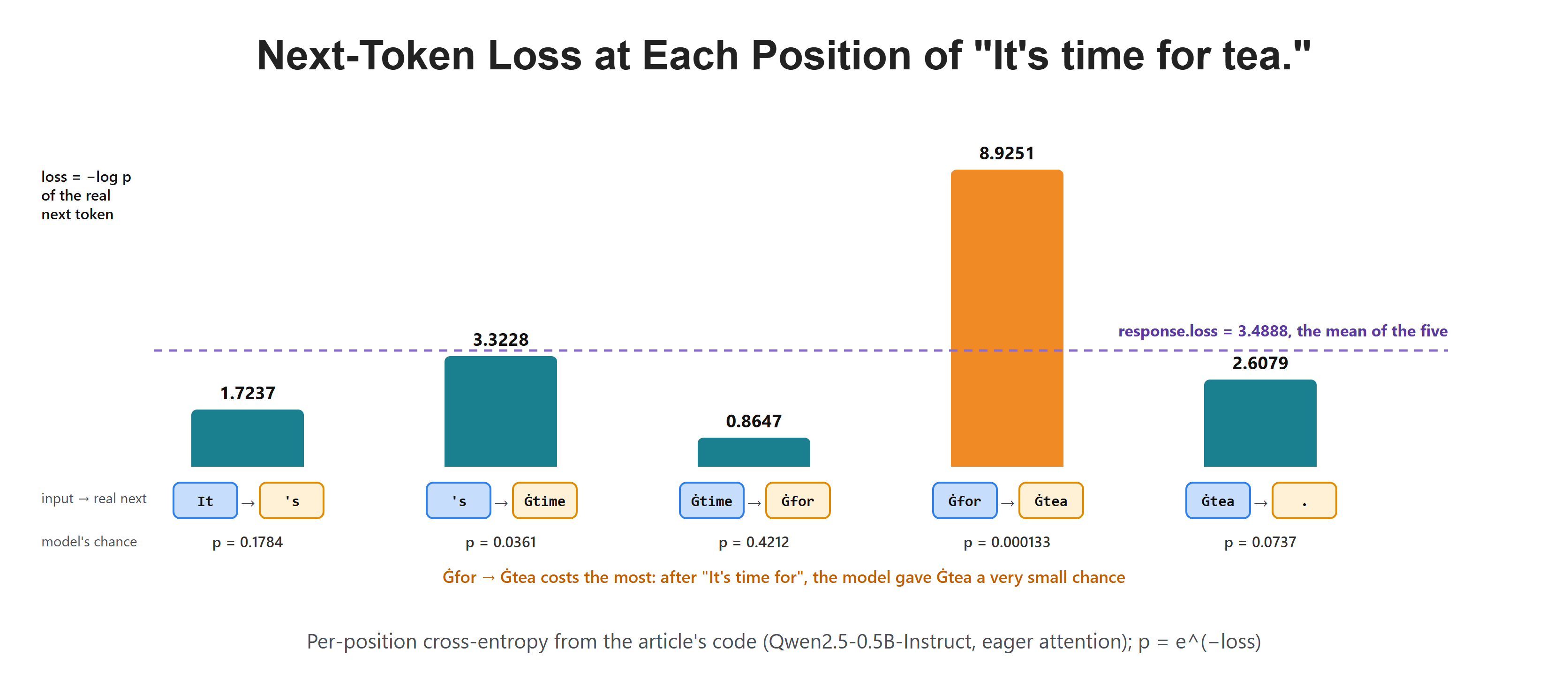
A decoder learns from plain text. Every position is a question with a known answer: what is the next token? The loss is the negative log of the probability the model gave to the real next token, averaged over the positions:
Where:
- : the token at position
- : the probability the model gives the real next token
- : the number of predictions, one fewer than the number of tokens
The figure below shows this loss on our first sentence, "It's time for tea." There is one loss for each token and the real token after it, and the dashed line is their mean. Under each bar, the loss is turned back into the model's chance.
When we pass the input ids as labels, the model computes this loss for us.
x = tok("It's time for tea.", return_tensors="pt").to("cuda")
response = model(**x, labels=x["input_ids"])
response.losstensor(3.4888, device='cuda:0')The mean loss over our sentence is 3.4888. Let's see the loss at each position.
torch.nn.functional.cross_entropy(response.logits[0, :-1].float(), x["input_ids"][0, 1:], reduction="none")tensor([1.7237, 3.3228, 0.8647, 8.9251, 2.6079], device='cuda:0')Here, we can see 5 losses for 6 tokens. The fourth position, Ġfor → Ġtea, costs the most, 8.9251, because after "It's time for" the model gave Ġtea a very small chance. Training nudges the weights to raise the probability of the real next token at every position.
Conclusion
This is how Qwen2.5-0.5B works. We started with text, split it into 6 tokens and looked up their rows in a 151,936 × 896 table. We saw why a token needs attention, built self-attention, the causal mask, multi-head attention and cross-attention by hand, and found which of them Qwen uses. We followed the vectors through 24 decoder layers, each one an RMSNorm, grouped-query attention with RoPE, a second RMSNorm and a SwiGLU MLP, joined by residual adds. Finally, the shared LM head turned the last vector into 151,936 scores, and a loop of such passes wrote text.
Key takeaways:
- Attention is the only part of a decoder layer that mixes tokens, and Qwen2.5 uses causal self-attention only, with no cross-attention.
- Qwen2.5-0.5B keeps the decoder plan of the original Transformer but swaps the parts: RMSNorm, RoPE, grouped-query attention and SwiGLU.
- Grouped-query attention lets 14 query heads share 2 key-value heads, which cuts the KV cache from 84 KB to 12 KB per token.
- RoPE adds no weights: it rotates queries and keys so that attention scores depend on the distance between tokens.
- The MLPs hold 63.5% of the weights, and the shared embedding table holds another 27.6%.
Next steps:
- Read The Attention Formula: What Softmax and the Square Root of d Actually Do for the scaling step in depth.
- Read Transformer Architecture and Tokenization Explained for the basics of tokens, embeddings and attention.
- Read MHA vs MQA vs GQA: How Modern LLMs Shrink the KV Cache for more on grouped-query attention.
- See this model classify text in Laya 421M vs Qwen3.5 0.8B vs Qwen2.5 0.5B: Small Models for Text Classification.