Breast Cancer Detection Using CNN

Breast Cancer Detection Using CNN in Python

Breast cancer is the most commonly occurring cancer in women and the second most common cancer overall. There were over 2 million new cases in 2018, making it a significant health problem in present days.

The key challenge in breast cancer detection is to classify tumors as malignant or benign. Malignant refers to cancer cells that can invade and kill nearby tissue and spread to other parts of the body. A benign tumor, unlike a malignant one, does not spread and is safer. Deep neural network techniques can improve the accuracy of early diagnosis a lot.

In this blog, we will build a 1D CNN in TensorFlow to classify tumors as malignant or benign using the Wisconsin diagnostic dataset.

tensorflow 2.3 is used to build the model. Install it with this command.

PLAINTEXT

!pip install tensorflow-gpu==2.3.0-rc0

Importing necessary library that will use in model building.

PYTHON

import tensorflow as tf
from tensorflow import keras
from tensorflow.keras import Sequential
from tensorflow.keras.layers import Flatten, Dense, Dropout, BatchNormalization
from tensorflow.keras.layers import Conv1D, MaxPool1D

from tensorflow.keras.optimizers import Adam

print(tf.__version__)

OUTPUT

2.3.0

pandas for loading and manipulating the data.

NumPy is used for working with arrays. It also has functions for linear algebra, fourier transforms, and matrices.

pyplot from matplotlib is used to visualize the results.

Seaborn is a Python plotting library built on matplotlib. It makes it easy to draw clear statistical charts.

PYTHON

import pandas as pd
import numpy as np
import  seaborn as sns
import matplotlib.pyplot as plt

PYTHON

/usr/local/lib/python3.6/dist-packages/statsmodels/tools/_testing.py:19: FutureWarning: pandas.util.testing is deprecated. Use the functions in the public API at pandas.testing instead.
  import pandas.util.testing as tm

PYTHON

from sklearn import datasets, metrics
from sklearn.model_selection import train_test_split
from sklearn.preprocessing import StandardScaler

Load and return the breast cancer classification dataset. The breast cancer dataset is a classic and very easy binary classification dataset.

PYTHON

cancer = datasets.load_breast_cancer()

View any particular column with the help of cancer.DESCR.

PYTHON

print(cancer.DESCR)

PYTHON

.. _breast_cancer_dataset:

Breast cancer wisconsin (diagnostic) dataset
--------------------------------------------

**Data Set Characteristics:**

    :Number of Instances: 569

    :Number of Attributes: 30 numeric, predictive attributes and the class

    :Attribute Information:
        - radius (mean of distances from center to points on the perimeter)
        - texture (standard deviation of gray-scale values)
        - perimeter
        - area
        - smoothness (local variation in radius lengths)
        - compactness (perimeter^2 / area - 1.0)
        - concavity (severity of concave portions of the contour)
        - concave points (number of concave portions of the contour)
        - symmetry
        - fractal dimension ("coastline approximation" - 1)

        The mean, standard error, and "worst" or largest (mean of the three
        largest values) of these features were computed for each image,
        resulting in 30 features.  For instance, field 3 is Mean Radius, field
        13 is Radius SE, field 23 is Worst Radius.

        - class:
                - WDBC-Malignant
                - WDBC-Benign

    :Summary Statistics:

    ===================================== ====== ======
                                           Min    Max
    ===================================== ====== ======
    radius (mean):                        6.981  28.11
    texture (mean):                       9.71   39.28
    perimeter (mean):                     43.79  188.5
    area (mean):                          143.5  2501.0
    smoothness (mean):                    0.053  0.163
    compactness (mean):                   0.019  0.345
    concavity (mean):                     0.0    0.427
    concave points (mean):                0.0    0.201
    symmetry (mean):                      0.106  0.304
    fractal dimension (mean):             0.05   0.097
    radius (standard error):              0.112  2.873
    texture (standard error):             0.36   4.885
    perimeter (standard error):           0.757  21.98
    area (standard error):                6.802  542.2
    smoothness (standard error):          0.002  0.031
    compactness (standard error):         0.002  0.135
    concavity (standard error):           0.0    0.396
    concave points (standard error):      0.0    0.053
    symmetry (standard error):            0.008  0.079
    fractal dimension (standard error):   0.001  0.03
    radius (worst):                       7.93   36.04
    texture (worst):                      12.02  49.54
    perimeter (worst):                    50.41  251.2
    area (worst):                         185.2  4254.0
    smoothness (worst):                   0.071  0.223
    compactness (worst):                  0.027  1.058
    concavity (worst):                    0.0    1.252
    concave points (worst):               0.0    0.291
    symmetry (worst):                     0.156  0.664
    fractal dimension (worst):            0.055  0.208
    ===================================== ====== ======

    :Missing Attribute Values: None

    :Class Distribution: 212 - Malignant, 357 - Benign

A pandas DataFrame keeps all inputs and outputs together. The code below creates a dataframe from the cancer data and feature names.

PYTHON

X = pd.DataFrame(data = cancer.data, columns=cancer.feature_names)
X.head()

OUTPUT

	mean radius	mean texture	mean perimeter	mean area	mean smoothness	mean compactness	mean concavity	mean concave points	mean symmetry	mean fractal dimension	radius error	texture error	perimeter error	area error	smoothness error	compactness error	concavity error	concave points error	symmetry error	fractal dimension error	worst radius	worst texture	worst perimeter	worst area	worst smoothness	worst compactness	worst concavity	worst concave points	worst symmetry	worst fractal dimension
0	17.99	10.38	122.80	1001.0	0.11840	0.27760	0.3001	0.14710	0.2419	0.07871	1.0950	0.9053	8.589	153.40	0.006399	0.04904	0.05373	0.01587	0.03003	0.006193	25.38	17.33	184.60	2019.0	0.1622	0.6656	0.7119	0.2654	0.4601	0.11890
1	20.57	17.77	132.90	1326.0	0.08474	0.07864	0.0869	0.07017	0.1812	0.05667	0.5435	0.7339	3.398	74.08	0.005225	0.01308	0.01860	0.01340	0.01389	0.003532	24.99	23.41	158.80	1956.0	0.1238	0.1866	0.2416	0.1860	0.2750	0.08902
2	19.69	21.25	130.00	1203.0	0.10960	0.15990	0.1974	0.12790	0.2069	0.05999	0.7456	0.7869	4.585	94.03	0.006150	0.04006	0.03832	0.02058	0.02250	0.004571	23.57	25.53	152.50	1709.0	0.1444	0.4245	0.4504	0.2430	0.3613	0.08758
3	11.42	20.38	77.58	386.1	0.14250	0.28390	0.2414	0.10520	0.2597	0.09744	0.4956	1.1560	3.445	27.23	0.009110	0.07458	0.05661	0.01867	0.05963	0.009208	14.91	26.50	98.87	567.7	0.2098	0.8663	0.6869	0.2575	0.6638	0.17300
4	20.29	14.34	135.10	1297.0	0.10030	0.13280	0.1980	0.10430	0.1809	0.05883	0.7572	0.7813	5.438	94.44	0.011490	0.02461	0.05688	0.01885	0.01756	0.005115	22.54	16.67	152.20	1575.0	0.1374	0.2050	0.4000	0.1625	0.2364	0.07678

PYTHON

y = cancer.target

OUTPUT

y

array([0, 0, 0, 0, 0, 0, 0, 0, 0, 0, 0, 0, 0, 0, 0, 0, 0, 0, 0, 1, 1, 1,
       0, 0, 0, 0, 0, 0, 0, 0, 0, 0, 0, 0, 0, 0, 0, 1, 0, 0, 0, 0, 0, 0,
       0, 0, 1, 0, 1, 1, 1, 1, 1, 0, 0, 1, 0, 0, 1, 1, 1, 1, 0, 1, 0, 0...])

PYTHON

cancer.target_names

OUTPUT

array(['malignant', 'benign'], dtype='<U9')

PYTHON

X.shape

OUTPUT

(569, 30)

Manual splitting is impractical, and random splitting is important for generalization. train_test_split from scikit-learn handles this, putting 80% of the data into training and 20% into testing.

PYTHON

X_train, X_test, y_train, y_test = train_test_split(X, y, test_size = 0.2, random_state = 0, stratify = y)

PYTHON

X_train.shape

OUTPUT

(455, 30)

PYTHON

X_test.shape

OUTPUT

(114, 30)

StandardScaler removes the mean and scales the data to unit variance.

PYTHON

scaler = StandardScaler()
X_train = scaler.fit_transform(X_train)
X_test = scaler.transform(X_test)

PYTHON

X_train = X_train.reshape(455,30,1)
X_test = X_test.reshape(114, 30, 1)

Building the CNN Model

A Sequential() function is the easiest way to build a model in Keras. It lets us build a model layer by layer. Each layer has weights that correspond to the layer the follows it. Use the add() function to add layers to our model.

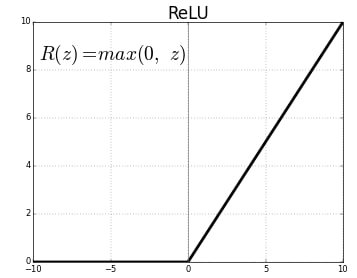
Conv1D() is a 1D convolution layer. It is good at pulling features from a fixed-length part of the data, when the exact spot of the feature does not matter. In the first Conv1D() layer, we learn 36 filters with a window size of 3. The input_shape gives the shape of the input, which the first layer of any neural network needs. We use the ReLU activation function here.

The Rectified Linear Unit (ReLU) is the most used activation function in deep learning. It returns 0 for any negative input, and for any positive value x it returns x. So we can write it as f(x)=max(0,x)

ReLU activation function graph showing zero output for negative inputs and linear output for positive values

To stop problem of shrinkage of data we use concept called Padding.

It has two types:

valid
same

Flattening is converting the data into a 1-dimensional array for inputting it to the next layer. The output of the convolutional layers is flattened to create a single long feature vector.

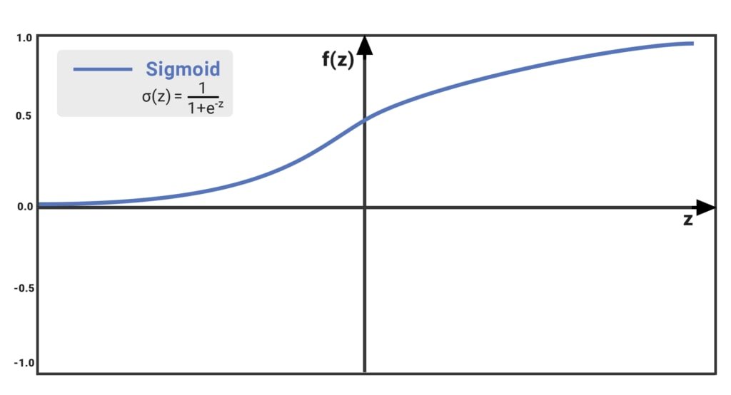
The Sigmoid function takes a value and returns another value between 0 and 1. It is non-linear and easy to work with. It is also smooth across all values of z and has a fixed output range.

Sigmoid activation function graph showing the S-curve mapping any input to a value between 0 and 1

PYTHON

epochs = 50
model = Sequential()
model.add(Conv1D(filters=32, kernel_size=2, activation='relu', input_shape = (30,1)))
model.add(BatchNormalization())
model.add(Dropout(0.2))

model.add(Conv1D(filters=64, kernel_size=2, activation='relu'))
model.add(BatchNormalization())
model.add(Dropout(0.5))

model.add(Flatten())
model.add(Dense(64, activation='relu'))
model.add(Dropout(0.5))

model.add(Dense(1, activation='sigmoid'))

PYTHON

model.summary()

PYTHON

Model: "sequential"
_________________________________________________________________
Layer (type)                 Output Shape              Param #
=================================================================
conv1d (Conv1D)              (None, 29, 32)            96
_________________________________________________________________
batch_normalization (BatchNo (None, 29, 32)            128
_________________________________________________________________
dropout (Dropout)            (None, 29, 32)            0
_________________________________________________________________
conv1d_1 (Conv1D)            (None, 28, 64)            4160
_________________________________________________________________
batch_normalization_1 (Batch (None, 28, 64)            256
_________________________________________________________________
dropout_1 (Dropout)          (None, 28, 64)            0
_________________________________________________________________
flatten (Flatten)            (None, 1792)              0
_________________________________________________________________
dense (Dense)                (None, 64)                114752
_________________________________________________________________
dropout_2 (Dropout)          (None, 64)                0
_________________________________________________________________
dense_1 (Dense)              (None, 1)                 65
=================================================================
Total params: 119,457
Trainable params: 119,265
Non-trainable params: 192
_________________________________________________________________

Compile defines the loss function, the optimizer, and the metrics. That's all. It has nothing to do with the weights, and we can compile a model as many times as we want without causing any problem to pretrained weights.

PLAINTEXT

model.compile(optimizer=Adam(lr=0.00005), loss = 'binary_crossentropy', metrics=['accuracy'])

Trains the model for a fixed number of epochs (iterations on a dataset).

PYTHON

history = model.fit(X_train, y_train, epochs=epochs, validation_data=(X_test, y_test), verbose=1)

OUTPUT

...
Epoch 46/50
15/15 [==============================] - 0s 6ms/step - loss: 0.1054 - accuracy: 0.9560 - val_loss: 0.1064 - val_accuracy: 0.9649
Epoch 47/50
15/15 [==============================] - 0s 6ms/step - loss: 0.1373 - accuracy: 0.9473 - val_loss: 0.1074 - val_accuracy: 0.9649
Epoch 48/50
15/15 [==============================] - 0s 7ms/step - loss: 0.1078 - accuracy: 0.9538 - val_loss: 0.1068 - val_accuracy: 0.9649
Epoch 49/50
15/15 [==============================] - 0s 6ms/step - loss: 0.0896 - accuracy: 0.9648 - val_loss: 0.1060 - val_accuracy: 0.9649
Epoch 50/50
15/15 [==============================] - 0s 6ms/step - loss: 0.0927 - accuracy: 0.9648 - val_loss: 0.1047 - val_accuracy: 0.9649

PYTHON

def plot_learningCurve(history, epoch):
  # Plot training & validation accuracy values
  epoch_range = range(1, epoch+1)
  plt.plot(epoch_range, history.history['accuracy'])
  plt.plot(epoch_range, history.history['val_accuracy'])
  plt.title('Model accuracy')
  plt.ylabel('Accuracy')
  plt.xlabel('Epoch')
  plt.legend(['Train', 'Val'], loc='upper left')
  plt.show()

  # Plot training & validation loss values
  plt.plot(epoch_range, history.history['loss'])
  plt.plot(epoch_range, history.history['val_loss'])
  plt.title('Model loss')
  plt.ylabel('Loss')
  plt.xlabel('Epoch')
  plt.legend(['Train', 'Val'], loc='upper left')
  plt.show()

A history object that contains all information collected during training.

PYTHON

history.history

OUTPUT

{'accuracy': [0.6197802424430847, 0.7494505643844604, 0.795604407787323, 0.8461538553237915, 0.8395604491233826, 0.8593406677246094, 0.8901098966598511, 0.8791208863258362, 0.8813186883926392, 0.9098901152610779, 0.903296709060669, 0.9230769276618958, ...]}

PYTHON

plot_learningCurve(history, epochs)

In the Model accuracy graph, validation accuracy is always greater than train accuracy, which means the model is not overfitting.

In the Model accuracy graph, validation loss is also lower than training loss. The model can keep training until validation loss rises above training loss.

The 1D CNN successfully classifies breast cancer with good generalization on the Wisconsin diagnostic dataset.

Conclusion

In this blog, we built a 1D CNN to detect breast cancer using the Wisconsin diagnostic dataset. We split 569 samples into train and test sets and applied StandardScaler normalization. The two-block convolutional model trained with Adam reached about 96.5% test accuracy in 50 epochs.

Key takeaways:

A lightweight 1D CNN with Conv1D, BatchNormalization, and Dropout can achieve strong accuracy on small medical datasets without overfitting.
BatchNormalization stabilizes training by keeping layer activations near zero mean and unit variance, which lets us use a lower learning rate safely.
Validation accuracy consistently higher than training accuracy is a healthy sign: Dropout is working as intended, and the model generalizes well to unseen samples.

Next steps:

Compare 1D CNN performance against a fully connected ANN on the same dataset in Building Your First ANN with TensorFlow 2.0.
Apply the same Conv1D approach to time-series data in Human Activity Recognition with Accelerometer Data.
Experiment with increasing epochs to 100 or adding a third convolutional block to push test accuracy closer to 98%.